Getting Started with irtQ

What is irtQ?

irtQ is an R package for unidimensional Item Response Theory (IRT) analyses. It supports mixed-format tests containing both dichotomous and polytomous items, and provides a unified interface for the most common psychometric tasks in educational and psychological measurement.

Why IRT? A Brief Motivation

Before using irtQ, it helps to understand why IRT is preferred over Classical Test Theory (CTT) for many measurement tasks.

Classical Test Theory (CTT) summarizes examinees by their total (or proportion) correct score and items by their observed difficulty (p-value) and point-biserial correlation. While straightforward, CTT has well-known limitations:

Sample dependence: item statistics (difficulty, discrimination) change with the examinee group, and person scores change with the item set
No item-level probability model: CTT does not tell us the probability that a specific person answers a specific item correctly
Limited equating: comparing scores across different test forms requires strong assumptions

Item Response Theory (IRT) addresses these limitations by modeling the probability of each response as a function of a latent trait $\theta$ (ability, proficiency, or attitude) and item parameters. Key advantages are:

Invariance: item parameters do not depend on the ability distribution of the calibration sample; person parameters do not depend on which particular items were administered
Item-level modeling: each item has its own characteristic curve describing how response probability changes with $\theta$
Common scale: items and persons are placed on the same $\theta$ continuum, enabling equating, adaptive testing, and longitudinal measurement

Core Capabilities of irtQ

irtQ covers the full IRT workflow:

Primary functions:

Estimating item parameters — fixed-form calibration, pretest calibration using Fixed Item Parameter Calibration (FIPC) and Fixed Ability Parameter Calibration (FAPC) approaches, and multiple-group calibration (est_irt(), est_mg(), est_item())
Estimating examinee abilities — maximum likelihood (ML), weighted likelihood (WLE), maximum a posteriori (MAP), expected a posteriori (EAP), EAP summed scoring, and inverse test characteristic curve (TCC) scoring (est_score())
Evaluating item-level model–data fit — $\chi^2$ , $G^2$ , infit/outfit, $S$ - $X^2$ (irtfit(), sx2_fit())
Detecting differential item functioning (DIF) — residual-based DIF (RDIF), generalized residual-based DIF (GRDIF), and simultaneous item bias test modified for CAT (CATSIB) (rdif(), grdif(), catsib())
Computing classification accuracy and consistency indices (cac_lee(), cac_rud())

Utilities:

Function	Purpose
`simdat()`	Simulate IRT item response data
`info()`	Item and test information functions
`traceline()`	Item and test characteristic curves
`lwrc()`	Lord–Wingersky recursion (summed-score distributions)
`gen.weight()`	Generate quadrature weights from a distribution
`covirt()`	IRT-based covariance between items
`run_flexmirt()`	Run flexMIRT directly from R

This vignette introduces the IRT models supported by irtQ and the item metadata data structure that connects all functions. At the end, a minimal end-to-end workflow ties everything together.

Installation

Install the released version from CRAN:

install.packages("irtQ")

Install the development version from GitHub:

# install.packages("devtools")
devtools::install_github("hwangQ/irtQ")

Load the package:

library(irtQ)

Supported IRT Models

irtQ supports the following unidimensional IRT models for dichotomous and polytomous items.

Dichotomous Models: 1PLM, 2PLM, and 3PLM

For a binary response $Y \in \{0, 1\}$ from an examinee with latent ability $\theta$ , the probability of a correct response ( $Y = 1$ ) under the three-parameter logistic model (3PLM) is:

$P(Y = 1 \mid \theta) = g + \frac{1 - g}{1 + \exp(-D\,a\,(\theta - b))}$

The four quantities in this equation each have a concrete interpretation:

$\theta$ — Latent ability (person parameter)
The unobserved trait being measured. The $\theta$ scale is typically standardized so that $\theta \sim N(0, 1)$ in the reference population: $\theta = 0$ is average ability, $\theta = 1$ is one standard deviation above average, and so on.

$a$ — Discrimination (item parameter)
Controls how steeply the item characteristic curve (ICC) rises. A highly discriminating item (large $a$ ) sharply separates examinees just below and just above the item’s difficulty; a weakly discriminating item (small $a$ ) produces a nearly flat ICC and provides little information about $\theta$ . In practice, $a$ typically ranges from about 0.5 to 2.5.

$b$ — Difficulty (item parameter)
The point on the $\theta$ scale where the probability of a correct response is halfway between $g$ and 1, i.e. $P = g + (1-g)/2$ . For the 2PLM (where $g = 0$ ), this simplifies to the $\theta$ value where $P = 0.5$ . Items with $b < 0$ are easy (most examinees answer correctly); items with $b > 0$ are hard. Values typically range from about $-3$ to $+3$ .

$g$ — Pseudo-guessing (item parameter)
The lower asymptote of the ICC — the probability of a correct response as $\theta \to -\infty$ . For a 5-option multiple-choice item with pure random guessing, $g = 0.2$ . When $g = 0$ the ICC passes through the origin and the model reduces to the 2PLM or 1PLM.

$D$ — Scaling constant
$D = 1.702$ is a constant that makes the logistic function closely approximate the normal ogive used in the original IRT formulation. Using $D = 1.702$ is conventional when working with logistic models; set $D = 1$ to work on the purely logistic scale. All irtQ functions accept D as an argument with default 1.702.

Special cases: 1PLM and 2PLM

Model	Discrimination	Guessing	Free parameters
1PLM	Fixed to 1 or constrained equal across items	$g = 0$	$b$ only
2PLM	Freely estimated, varies across items	$g = 0$	$a$ , $b$
3PLM	Freely estimated, varies across items	Freely estimated	$a$ , $b$ , $g$

Note on 1PLM in irtQ. When fix.a.1pl = TRUE (in est_irt()), the discrimination is fixed to the value a.val.1pl (default 1) — this is the strict Rasch model. When fix.a.1pl = FALSE (the default), the common discrimination is estimated from the data but constrained to be equal across all 1PLM items. Both specifications produce only $b$ as the item-differentiating parameter, but the second is more flexible when the Rasch assumption of $a = 1$ does not exactly hold.

Polytomous Models: GRM and GPCM

For items with $K$ ordered response categories scored $0, 1, \ldots, K-1$ (e.g., a 4-point rating scale scored 0–3), irtQ supports two models.

Graded Response Model (GRM)

The GRM (Samejima, 1969) models $K - 1$ cumulative boundary response functions, one for each adjacent pair of categories. The cumulative probability of responding in category $k$ or higher is:

$P^*(Y \ge k \mid \theta) = \frac{1}{1 + \exp(-D\,a\,(\theta - b_k))}, \quad k = 1, \ldots, K-1$

with the conventions $P^*(Y \ge 0) = 1$ and $P^*(Y \ge K) = 0$ .

The probability of responding in exactly category $k$ is then:

$P(Y = k \mid \theta) = P^*(Y \ge k \mid \theta) - P^*(Y \ge k+1 \mid \theta)$

Parameters:

$a$ : a single discrimination parameter shared across all category boundaries
$b_1 < b_2 < \cdots < b_{K-1}$ : ordered threshold parameters, where $b_k$ is the $\theta$ value at which the probability of responding above category $k-1$ equals 0.5. The ordering constraint ensures that the response probabilities are non-negative for all $\theta$ .

Intuition: Think of the GRM as applying a 2PLM-like curve to each of the $K-1$ adjacent-category boundaries. $b_1$ marks the easy end of the scale (where most examinees move from category 0 to category 1), and $b_{K-1}$ marks the hard end (where examinees move into the top category).

Example (4-category GRM item, $K = 4$ ):

$b_1 = -1.5$ : Examinees with $\theta \approx -1.5$ have a 50% chance of scoring 1 or higher
$b_2 = 0.0$ : Examinees with $\theta \approx 0$ have a 50% chance of scoring 2 or higher
$b_3 = 1.2$ : Examinees with $\theta \approx 1.2$ have a 50% chance of scoring 3 (the top category)

Generalized Partial Credit Model (GPCM)

The GPCM (Muraki, 1992) generalizes the Partial Credit Model [PCM; Masters (1982)] by allowing items to have different discrimination parameters. The probability of responding in category $k$ is:

$P(Y = k \mid \theta) = \frac{\exp\!\left(\displaystyle\sum_{v=0}^{k} D\,a\,(\theta - b_v)\right)} {\displaystyle\sum_{h=0}^{K-1} \exp\!\left(\displaystyle\sum_{v=0}^{h} D\,a\,(\theta - b_v)\right)}$

where the convention $b_0 = 0$ is used so that the numerator for $k = 0$ simplifies to $\exp(0) = 1$ .

Parameters:

$a$ : a single discrimination parameter for the item
$b_1, b_2, \ldots, b_{K-1}$ : step parameters (also called threshold parameters), where $b_v$ governs the transition from category $v-1$ to category $v$ . Unlike GRM thresholds, GPCM step parameters need not be ordered.

Relationship to other models:

Setting $a = 1$ for all items gives the Partial Credit Model (PCM) (Masters, 1982)
The GPCM is therefore a generalization of the PCM that allows item-varying discrimination

How to specify in irtQ: For an item with $K$ categories, provide a vector of $K - 1$ step parameters as the d argument in shape_df(). The convention $b_0 = 0$ is handled internally; you do not supply $b_0$ .

Summary: All Supported Models

Model	Item type	Parameters	Notes
1PLM	Dichotomous	$b$	$a$ fixed or equal-constrained; $g = 0$
2PLM	Dichotomous	$a,\, b$	$g = 0$
3PLM	Dichotomous	$a,\, b,\, g$	All three parameters free
GRM	Polytomous	$a,\, b_1, \ldots, b_{K-1}$	Thresholds must be ordered
GPCM	Polytomous	$a,\, b_1, \ldots, b_{K-1}$	Step params need not be ordered
PCM	Polytomous	$b_1, \ldots, b_{K-1}$	GPCM with $a = 1$

Alias: "DRM" is accepted as a model string for any dichotomous item (1PLM, 2PLM, or 3PLM) in contexts where the model is already encoded in the metadata.

Item Metadata: The Central Data Structure

Nearly every irtQ function accepts a data frame x as its first argument. This item metadata frame is a standardized, row-per-item table that encodes the IRT model and parameter values for each item in a test form. It serves as the single input format shared across all analyses — calibration, scoring, fit evaluation, DIF detection, and more — so you only need to build it once.

Column Structure

Column	Type	Description
`id`	character	Unique item identifier
`cats`	integer	Number of response categories (2 for dichotomous)
`model`	character	IRT model: `"1PLM"`, `"2PLM"`, `"3PLM"`, `"GRM"`, `"GPCM"`
`par.1`	numeric	Discrimination parameter ( $a$ )
`par.2`	numeric	Difficulty ( $b$ ) for dichotomous; first threshold ( $b_1$ ) for polytomous
`par.3`	numeric	Guessing ( $g$ ) for 3PLM; second threshold ( $b_2$ ) for polytomous; `NA` otherwise
`par.4`, …	numeric	Additional thresholds for polytomous items; `NA` for dichotomous

The number of par.* columns grows with the maximum number of categories across items. For example, a test containing a GRM item with 5 categories will have columns par.1 through par.5, with NA filling unused slots for dichotomous items.

A Concrete Example

# 3 dichotomous items (2PLM) + 2 polytomous items (GRM, 4 categories)
meta_demo <- shape_df(
  par.drm = list(
    a = c(1.2, 0.9, 1.5),
    b = c(-0.5, 0.0, 1.0),
    g = c(NA, NA, NA)         # NA: no guessing for 2PLM
  ),
  par.prm = list(
    a = c(1.8, 1.3),
    d = list(
      c(-1.2, 0.0, 1.2),      # 3 thresholds for item 4 (4 categories)
      c(-0.8, 0.3, 1.5)       # 3 thresholds for item 5 (4 categories)
    )
  ),
  item.id = paste0("I", 1:5),
  cats    = c(2, 2, 2, 4, 4),
  model   = c("2PLM", "2PLM", "2PLM", "GRM", "GRM")
)
meta_demo
#>   id cats model par.1 par.2 par.3 par.4
#> 1 I1    2  2PLM   1.2  -0.5    NA    NA
#> 2 I2    2  2PLM   0.9   0.0    NA    NA
#> 3 I3    2  2PLM   1.5   1.0    NA    NA
#> 4 I4    4   GRM   1.8  -1.2   0.0   1.2
#> 5 I5    4   GRM   1.3  -0.8   0.3   1.5

Reading across the columns:

Items I1–I3 are 2PLM: par.1 = $a$ , par.2 = $b$ , par.3 = NA (no guessing), par.4 = NA (no third threshold)
Items I4–I5 are GRM with 4 categories: par.1 = $a$ , par.2–par.4 = $b_1, b_2, b_3$

Creating Item Metadata with `shape_df()`

shape_df() is the primary tool for building item metadata from scratch. It takes parameter values as named lists and returns a correctly formatted metadata data frame.

Example 1: Six dichotomous items (1PLM, 2PLM, 3PLM mixed)

meta_ex1 <- shape_df(
  par.drm = list(
    a = c(1.0, 1.0, 0.9, 1.2, 0.8, 2.1),     # discrimination
    b = c(0.2, 2.3, -0.4, -2.5, 0.9, 1.2),   # difficulty
    g = c(NA,  NA,   NA,   NA,  0.2, 0.1)     # guessing: NA for 1PLM/2PLM
  ),
  item.id = paste0("ITEM", 1:6),
  cats  = 2,
  model = c("1PLM", "1PLM", "2PLM", "2PLM", "3PLM", "3PLM")
)
meta_ex1
#>      id cats model par.1 par.2 par.3
#> 1 ITEM1    2  1PLM   1.0   0.2    NA
#> 2 ITEM2    2  1PLM   1.0   2.3    NA
#> 3 ITEM3    2  2PLM   0.9  -0.4    NA
#> 4 ITEM4    2  2PLM   1.2  -2.5    NA
#> 5 ITEM5    2  3PLM   0.8   0.9   0.2
#> 6 ITEM6    2  3PLM   2.1   1.2   0.1

Key points:

par.drm takes a named list with three vectors: a (discrimination), b (difficulty), and g (guessing). Set g = NA for 1PLM and 2PLM items.
Items 1 and 2 are 1PLM: their a values are provided in par.drm but will be handled according to the fix.a.1pl argument in estimation functions. The par.3 column in the output is NA because there is no guessing for 1PLM items.
Items 5 and 6 are 3PLM: their guessing parameters are 0.2 and 0.1 respectively.

Example 2: Mixed-format test (dichotomous + polytomous)

meta_ex2 <- shape_df(
  par.drm = list(
    a = c(0.8, 2.1),
    b = c(0.9, 1.2),
    g = c(0.2, 0.1)
  ),
  par.prm = list(
    a = c(1.9, 1.3, 0.7),
    d = list(
      c(-1.20, -0.52,  0.25),       # GRM  item: 4 categories → 3 thresholds
      c(-2.20, -1.50, -0.55),       # GPCM item: 4 categories → 3 step params
      c(-0.92, -0.43,  0.49, 1.11)  # GPCM item: 5 categories → 4 step params
    )
  ),
  item.id = paste0("ITEM", 1:5),
  cats  = c(2, 2, 4, 4, 5),
  model = c("3PLM", "3PLM", "GRM", "GPCM", "GPCM")
)
meta_ex2
#>      id cats model par.1 par.2 par.3 par.4 par.5
#> 1 ITEM1    2  3PLM   0.8  0.90  0.20    NA    NA
#> 2 ITEM2    2  3PLM   2.1  1.20  0.10    NA    NA
#> 3 ITEM3    4   GRM   1.9 -1.20 -0.52  0.25    NA
#> 4 ITEM4    4  GPCM   1.3 -2.20 -1.50 -0.55    NA
#> 5 ITEM5    5  GPCM   0.7 -0.92 -0.43  0.49  1.11

Key points:

par.prm takes a named list with a (discrimination for polytomous items) and d (a list of threshold/step parameter vectors, one per polytomous item).
Each vector in d must have length $K - 1$ where $K$ is cats for that item: 4-category items need 3 values; 5-category items need 4 values.
For a GRM item, the values in d are thresholds $b_1, \ldots, b_{K-1}$ , which must be in increasing order.
For a GPCM item, the values in d are step parameters $b_1, \ldots, b_{K-1}$ , which need not be ordered.
The d vectors for GRM and GPCM items can be mixed within the same par.prm list — the model argument determines which model applies to each item.

Example 3: Uniform model, auto-assigned IDs

When all items share the same model, a single model string is recycled. If item.id is omitted, IDs are auto-assigned as V1, V2, …

meta_ex3 <- shape_df(
  par.drm = list(
    a = c(1.0, 1.0, 0.9, 1.2, 0.8, 2.1),
    b = c(0.2, 2.3, -0.4, -2.5, 0.9, 1.2),
    g = c(0.1, 0.3, 0.1, 0.2, 0.2, 0.1)
  ),
  cats  = 2,
  model = "3PLM"   # recycled for all six items
)
meta_ex3
#>   id cats model par.1 par.2 par.3
#> 1 V1    2  3PLM   1.0   0.2   0.1
#> 2 V2    2  3PLM   1.0   2.3   0.3
#> 3 V3    2  3PLM   0.9  -0.4   0.1
#> 4 V4    2  3PLM   1.2  -2.5   0.2
#> 5 V5    2  3PLM   0.8   0.9   0.2
#> 6 V6    2  3PLM   2.1   1.2   0.1

Example 4: Default parameters (`default.par = TRUE`)

Set default.par = TRUE to create a metadata frame with placeholder parameters without specifying values explicitly. This is useful when you want to calibrate items from scratch and only need the structure, or as a starting point for editing. Default values are $a = 1$ , $b = 0$ , $g = 0.2$ for 3PLM and NA for 1PLM/2PLM; polytomous thresholds default to all zeros.

meta_ex4 <- shape_df(
  cats        = 2,
  model       = c("1PLM", "2PLM", "2PLM", "3PLM", "3PLM"),
  default.par = TRUE
)
meta_ex4
#>   id cats model par.1 par.2 par.3
#> 1 V1    2  1PLM     1     0    NA
#> 2 V1    2  2PLM     1     0    NA
#> 3 V1    2  2PLM     1     0    NA
#> 4 V1    2  3PLM     1     0     0
#> 5 V1    2  3PLM     1     0     0

`shape_df()` Argument Summary

Argument	Description
`par.drm`	Named list with `a`, `b`, `g` vectors for dichotomous items
`par.prm`	Named list with `a` and `d` (list of threshold vectors) for polytomous items
`item.id`	Character vector of item IDs; auto-assigned as `V1`, `V2`, … if omitted
`cats`	Integer vector of category counts per item (scalar if all equal)
`model`	Character vector of model strings (scalar if all equal)
`default.par`	If `TRUE`, fill parameters with built-in defaults (default `FALSE`)

Importing Item Metadata from External IRT Software

The bring.*() family of functions converts output files from external IRT programs into irtQ’s item metadata format. This makes it easy to use parameters calibrated in another program as the starting point for downstream irtQ analyses.

Each function returns a list; the $full_df component contains the complete standardized metadata data frame.

Importing from flexMIRT

# Locate the sample flexMIRT -prm.txt file bundled with irtQ
flex_file <- system.file("extdata", "flexmirt_sample-prm.txt", package = "irtQ")

# Import: returns a list keyed by group (e.g., Group1, Group2, ...)
meta_flex <- bring.flexmirt(file = flex_file, type = "par")$Group1$full_df
meta_flex
#>       id cats model     par.1       par.2        par.3      par.4      par.5
#> 1   CMC1    2  3PLM 0.7627842  1.46195307  0.261505353         NA         NA
#> 2   CMC2    2  3PLM 1.9212842 -1.04997761  0.175294361         NA         NA
#> 3   CMC3    2  3PLM 0.9266599  0.39475508  0.099746565         NA         NA
#> 4   CMC4    2  3PLM 1.0526419 -0.40704222  0.201193373         NA         NA
#> 5   CMC5    2  3PLM 0.8663350 -0.12481696  0.160420403         NA         NA
#> 6   CMC6    2  3PLM 1.6956204  0.62610659  0.072168572         NA         NA
#> 7   CMC7    2  3PLM 0.9061455  1.01573864  0.119458135         NA         NA
#> 8   CMC8    2  3PLM 0.8442812  0.80047702  0.114479251         NA         NA
#> 9   CMC9    2  3PLM 0.8541021  0.85236906  0.255248657         NA         NA
#> 10 CMC10    2  3PLM 1.5320152  0.09036640  0.135385451         NA         NA
#> 11 CMC11    2  3PLM 1.0018535 -0.46145320  0.132401405         NA         NA
#> 12 CMC12    2  3PLM 0.8784359  1.18144944  0.087687982         NA         NA
#> 13 CMC13    2  3PLM 1.4566944  1.40553715  0.181275480         NA         NA
#> 14 CMC14    2  3PLM 1.5142828  0.18435004  0.248064790         NA         NA
#> 15 CMC15    2  3PLM 1.2965707 -0.22914423  0.111920040         NA         NA
#> 16 CMC16    2  3PLM 2.0469491 -0.08536470  0.050890225         NA         NA
#> 17 CMC17    2  3PLM 1.3978190 -0.13421645  0.178526460         NA         NA
#> 18 CMC18    2  3PLM 1.6957073  1.24709400  0.273106846         NA         NA
#> 19 CMC19    2  3PLM 2.3117795 -1.01102523  0.179638721         NA         NA
#> 20 CMC20    2  3PLM 1.4489340 -1.65436976  0.190693574         NA         NA
#> 21 CMC21    2  3PLM 1.6281382 -1.19437963  0.121929251         NA         NA
#> 22 CMC22    2  3PLM 0.8320715 -0.67723050  0.197432042         NA         NA
#> 23 CMC23    2  3PLM 0.9768588 -0.25632988  0.130014303         NA         NA
#> 24 CMC24    2  3PLM 1.1418671  1.67963811  0.254011205         NA         NA
#> 25 CMC25    2  3PLM 0.7944843 -1.39426607  0.264555718         NA         NA
#> 26 CMC26    2  3PLM 1.0923706 -1.84806805  0.166491117         NA         NA
#> 27 CMC27    2  3PLM 1.1730201  0.07444365  0.131922668         NA         NA
#> 28 CMC28    2  3PLM 2.1546851 -0.08787145  0.208148649         NA         NA
#> 29 CMC29    2  3PLM 1.2810740 -1.38040199  0.201295671         NA         NA
#> 30 CMC30    2  3PLM 1.3505976  0.82351324  0.323145357         NA         NA
#> 31 CMC31    2  3PLM 0.8203985  0.70908638  0.082856907         NA         NA
#> 32 CMC32    2  3PLM 1.5235060 -0.88999000  0.257420730         NA         NA
#> 33 CMC33    2  3PLM 1.2711786 -1.31320312  0.186172388         NA         NA
#> 34 CMC34    2  3PLM 1.3107828  0.18690381  0.158109796         NA         NA
#> 35 CMC35    2  3PLM 1.4665995 -0.13801287  0.226328899         NA         NA
#> 36 CMC36    2  3PLM 0.8918806  1.09548554  0.126283949         NA         NA
#> 37 CMC37    2  3PLM 1.7287653 -0.40939097  0.104544594         NA         NA
#> 38 CMC38    2  3PLM 0.7327085 -0.37360246  0.218883035         NA         NA
#> 39  CFR1    5   GRM 1.9134815 -1.86983653 -1.238979525 -0.7140496 -0.2301269
#> 40  CFR2    5   GRM 1.2784658 -0.72406919 -0.068767894  0.5689640  1.0726913
#> 41  AMC1    2  3PLM 1.4655489  0.64088029  0.225388960         NA         NA
#> 42  AMC2    2  3PLM 1.7609502 -1.52832130  0.158898368         NA         NA
#> 43  AMC3    2  3PLM 1.4430127  0.54078083  0.138825943         NA         NA
#> 44  AMC4    2  3PLM 0.9784240 -0.36582964  0.126958991         NA         NA
#> 45  AMC5    2  3PLM 0.9915383  2.37079859  0.164822203         NA         NA
#> 46  AMC6    2  3PLM 2.2732723  1.62427761  0.178409401         NA         NA
#> 47  AMC7    2  3PLM 1.2256893 -0.07172021  0.131317231         NA         NA
#> 48  AMC8    2  3PLM 1.6399644  0.16526401  0.182665802         NA         NA
#> 49  AMC9    2  3PLM 1.2090633  0.23974948  0.081366545         NA         NA
#> 50 AMC10    2  3PLM 1.3201851  1.33993665  0.079323850         NA         NA
#> 51 AMC11    2  3PLM 1.7372043 -0.99805101  0.246773029         NA         NA
#> 52 AMC12    2  3PLM 0.9746876 -0.72824708  0.223540392         NA         NA
#> 53  AFR1    5   GRM 1.1378595 -0.37401164  0.215487852  0.8485578  1.3826066
#> 54  AFR2    5   GRM 1.2333756 -2.07872217 -1.347637330 -0.7054699 -0.1163185
#> 55  AFR3    5   GRM 0.8762246 -0.75520683 -0.005929073  0.6650100  1.2474287

bring.flexmirt() returns a nested list keyed by group name. Use $Group1$full_df, $Group2$full_df, etc. to access each group’s metadata.

Importing from PARSCALE

# Locate the sample PARSCALE .PAR file bundled with irtQ
pscale_file <- system.file("extdata", "parscale_sample.PAR", package = "irtQ")

# Import item parameters
meta_pscale <- bring.parscale(file = pscale_file, type = "par")$full_df
meta_pscale
#>      id cats model   par.1    par.2    par.3    par.4    par.5
#> 1  0001    2   DRM 0.78668  1.45392  0.26424       NA       NA
#> 2  0002    2   DRM 1.95256 -1.03590  0.16790       NA       NA
#> 3  0003    2   DRM 0.92423  0.36744  0.08911       NA       NA
#> 4  0004    2   DRM 1.06017 -0.41665  0.19257       NA       NA
#> 5  0005    2   DRM 0.86593 -0.15680  0.14700       NA       NA
#> 6  0006    2   DRM 1.70781  0.62067  0.06983       NA       NA
#> 7  0007    2   DRM 0.91006  0.99884  0.11532       NA       NA
#> 8  0008    2   DRM 0.84174  0.77277  0.10594       NA       NA
#> 9  0009    2   DRM 0.86645  0.84402  0.25407       NA       NA
#> 10 0010    2   DRM 1.54383  0.08762  0.13141       NA       NA
#> 11 0011    2   DRM 1.00673 -0.47776  0.12047       NA       NA
#> 12 0012    2   DRM 0.87475  1.15744  0.08077       NA       NA
#> 13 0013    2   DRM 1.48901  1.39467  0.18195       NA       NA
#> 14 0014    2   DRM 1.53152  0.18416  0.24621       NA       NA
#> 15 0015    2   DRM 1.30079 -0.24027  0.10225       NA       NA
#> 16 0016    2   DRM 2.06064 -0.08604  0.04616       NA       NA
#> 17 0017    2   DRM 1.41035 -0.13591  0.17396       NA       NA
#> 18 0018    2   DRM 1.73702  1.23955  0.27421       NA       NA
#> 19 0019    2   DRM 2.35588 -0.99336  0.17489       NA       NA
#> 20 0020    2   DRM 1.47074 -1.64613  0.17122       NA       NA
#> 21 0021    2   DRM 1.65023 -1.18579  0.10906       NA       NA
#> 22 0022    2   DRM 0.83234 -0.71780  0.17873       NA       NA
#> 23 0023    2   DRM 0.97745 -0.28252  0.11614       NA       NA
#> 24 0024    2   DRM 1.19351  1.66222  0.25751       NA       NA
#> 25 0025    2   DRM 0.80015 -1.42399  0.24565       NA       NA
#> 26 0026    2   DRM 1.10754 -1.84767  0.14416       NA       NA
#> 27 0027    2   DRM 1.17525  0.06034  0.12368       NA       NA
#> 28 0028    2   DRM 2.17855 -0.08451  0.20623       NA       NA
#> 29 0029    2   DRM 1.29244 -1.39057  0.17961       NA       NA
#> 30 0030    2   DRM 1.37376  0.82118  0.32351       NA       NA
#> 31 0031    2   DRM 0.81518  0.67339  0.07125       NA       NA
#> 32 0032    2   DRM 1.54708 -0.87791  0.25249       NA       NA
#> 33 0033    2   DRM 1.28305 -1.32022  0.16690       NA       NA
#> 34 0034    2   DRM 1.31798  0.17924  0.15299       NA       NA
#> 35 0035    2   DRM 1.48301 -0.13656  0.22323       NA       NA
#> 36 0036    2   DRM 0.89426  1.07673  0.12151       NA       NA
#> 37 0037    2   DRM 1.74214 -0.40933  0.09754       NA       NA
#> 38 0038    2   DRM 0.73472 -0.40711  0.20611       NA       NA
#> 39 0039    5   GRM 1.94931 -1.82855 -1.21040 -0.69548 -0.22021
#> 40 0040    5   GRM 1.30020 -0.70553 -0.06094  0.56671  1.06264
#> 41 0041    2   DRM 1.48353  0.63767  0.22449       NA       NA
#> 42 0042    2   DRM 1.79481 -1.50864  0.14541       NA       NA
#> 43 0043    2   DRM 1.45567  0.53570  0.13648       NA       NA
#> 44 0044    2   DRM 0.98254 -0.38343  0.11552       NA       NA
#> 45 0045    2   DRM 1.05231  2.31660  0.16867       NA       NA
#> 46 0046    2   DRM 2.41144  1.60547  0.18062       NA       NA
#> 47 0047    2   DRM 1.23217 -0.08089  0.12396       NA       NA
#> 48 0048    2   DRM 1.65413  0.16364  0.17983       NA       NA
#> 49 0049    2   DRM 1.21099  0.22634  0.07378       NA       NA
#> 50 0050    2   DRM 1.33178  1.32871  0.07789       NA       NA
#> 51 0051    2   DRM 1.76740 -0.98230  0.24200       NA       NA
#> 52 0052    2   DRM 0.97768 -0.75322  0.20821       NA       NA
#> 53 0053    5   GRM 1.15715 -0.36099  0.21902  0.84214  1.36791
#> 54 0054    5   GRM 1.25620 -2.03425 -1.31648 -0.68590 -0.10716
#> 55 0055    5   GRM 0.89213 -0.73461  0.00167  0.66112  1.23362

Importing from BILOG-MG

# Import from a BILOG-MG .PAR output file (not run — replace with your path)
meta_bilog <- bring.bilog(file = "output/mytest.PAR", type = "par")$full_df

Importing from the mirt package

# Fit a model with mirt (not run)
# mirt_mod <- mirt::mirt(data = my_data, model = 1, itemtype = "2PL")

# Convert to irtQ metadata
# meta_mirt <- bring.mirt(x = mirt_mod)$full_df

Common Arguments for `bring.*()` Functions

All bring.*() functions share two main arguments:

Argument	Description
`file`	Path to the external software output file
`type`	`"par"` for item parameter estimates; `"sco"` for ability score estimates

In practice, replace system.file(...) with the actual path to your file:

meta <- bring.flexmirt(file = "output/my_calibration-prm.txt",
                       type = "par")$Group1$full_df

Reading Item Metadata from a CSV File

You can also prepare item metadata in a spreadsheet and read it into R as a CSV file, as long as the column structure matches the irtQ specification.

# Read item metadata from a CSV file (not run — replace with your path)
meta_csv <- read.csv("my_item_parameters.csv", stringsAsFactors = FALSE)

# Verify the structure
str(meta_csv)
head(meta_csv)

Ensure that:

Column names are exactly id, cats, model, par.1, par.2, par.3, …
id is character, cats is integer, model is character, par.* are numeric
Missing threshold or guessing parameters are coded as NA
GRM threshold columns (par.2, par.3, …) are in increasing order within each row

A Complete End-to-End Workflow

This vignette has focused on item metadata — the central data structure that connects all irtQ functions. To show how metadata fits into the broader analysis pipeline, the example below walks through a minimal end-to-end workflow: define item metadata → simulate responses → estimate item parameters → estimate abilities → check recovery. Each step beyond metadata creation is covered in depth in its own dedicated vignette (see What’s Next? at the end of this page).

The following example walks through the core irtQ workflow from start to finish: define item metadata → simulate responses → estimate item parameters → estimate abilities → check recovery.

set.seed(2026)

# ---- Step 1: Define item metadata (20-item mixed test) ----
# 15 dichotomous 2PLM items + 5 polytomous GRM items (4 categories)
meta_wf <- shape_df(
  par.drm = list(
    a = c(0.8, 1.2, 1.5, 0.9, 1.1, 1.3, 0.7, 1.0, 1.4, 0.85,
          1.1, 0.9, 1.2, 1.0, 1.3),
    b = c(-1.5, -1.0, -0.5, -0.2, 0.0, 0.2, 0.5, 0.8, 1.0, 1.5,
          -1.2, -0.8, -0.3, 0.1, 0.4),
    g = rep(NA, 15)
  ),
  par.prm = list(
    a = c(1.4, 1.1, 0.9, 1.2, 1.0),
    d = list(
      c(-1.5, -0.2,  0.9),
      c(-1.2,  0.1,  1.2),
      c(-0.9,  0.4,  1.5),
      c(-1.1, -0.1,  1.0),
      c(-1.3,  0.3,  1.3)
    )
  ),
  item.id = c(paste0("D", 1:15), paste0("P", 1:5)),
  cats    = c(rep(2, 15), rep(4, 5)),
  model   = c(rep("2PLM", 15), rep("GRM", 5))
)

# ---- Step 2: Simulate response data (500 examinees, N(0,1)) ----
theta_true <- rnorm(500, mean = 0, sd = 1)
resp <- simdat(x = meta_wf, theta = theta_true, D = 1.702)

cat("Response matrix dimensions:", dim(resp), "\n")  # 500 examinees × 20 items
#> Response matrix dimensions: 500 20

# ---- Step 3: Estimate item parameters with est_irt() ----
mod <- est_irt(
  data    = resp,
  D       = 1.702,
  model   = c(rep("2PLM", 15), rep("GRM", 5)),
  cats    = c(rep(2, 15), rep(4, 5)),
  item.id = c(paste0("D", 1:15), paste0("P", 1:5)),
  EmpHist = FALSE,
  Etol    = 0.001,
  MaxE    = 300,
  se      = TRUE,
  verbose = FALSE
)

# Summarize calibration results
summary(mod)
#> 
#> Call:
#> est_irt(data = resp, D = 1.702, model = c(rep("2PLM", 15), rep("GRM", 
#>     5)), cats = c(rep(2, 15), rep(4, 5)), item.id = c(paste0("D", 
#>     1:15), paste0("P", 1:5)), EmpHist = FALSE, Etol = 0.001, 
#>     MaxE = 300, se = TRUE, verbose = FALSE)
#> 
#> Summary of the Data 
#>  Number of Items: 20
#>  Number of Cases: 500
#> 
#> Summary of Estimation Process 
#>  Maximum number of EM cycles: 300
#>  Convergence criterion of E-step: 0.001
#>  Number of rectangular quadrature points: 49
#>  Minimum & Maximum quadrature points: -6, 6
#>  Number of free parameters: 50
#>  Number of fixed items: 0
#>  Number of E-step cycles completed: 14
#>  Maximum parameter change: 0.000805268
#> 
#> Processing time (in seconds) 
#>  EM algorithm: 0.46
#>  Standard error computation: 0.02
#>  Total computation: 0.51
#> 
#> Convergence and Stability of Solution 
#>  First-order test: Convergence criteria are satisfied.
#>  Second-order test: Solution is a possible local maximum.
#>  Computation of variance-covariance matrix: 
#>   Variance-covariance matrix of item parameter estimates is obtainable.
#> 
#> Summary of Estimation Results 
#>  -2loglikelihood: 12453.76
#>  Akaike Information Criterion (AIC): 12553.76
#>  Bayesian Information Criterion (BIC): 12764.5
#>  Item Parameters: 
#>      id  cats  model  par.1  se.1  par.2  se.2  par.3  se.3  par.4  se.4
#> 1    D1     2   2PLM   1.01  0.12  -1.38  0.13     NA    NA     NA    NA
#> 2    D2     2   2PLM   1.33  0.17  -1.02  0.09     NA    NA     NA    NA
#> 3    D3     2   2PLM   1.64  0.19  -0.37  0.06     NA    NA     NA    NA
#> 4    D4     2   2PLM   0.95  0.10  -0.19  0.08     NA    NA     NA    NA
#> 5    D5     2   2PLM   1.10  0.12   0.05  0.07     NA    NA     NA    NA
#> 6    D6     2   2PLM   1.60  0.17   0.05  0.06     NA    NA     NA    NA
#> 7    D7     2   2PLM   0.64  0.08   0.49  0.11     NA    NA     NA    NA
#> 8    D8     2   2PLM   1.14  0.14   0.72  0.08     NA    NA     NA    NA
#> 9    D9     2   2PLM   1.69  0.23   0.83  0.07     NA    NA     NA    NA
#> 10  D10     2   2PLM   0.85  0.12   1.43  0.15     NA    NA     NA    NA
#> 11  D11     2   2PLM   1.12  0.16  -1.24  0.12     NA    NA     NA    NA
#> 12  D12     2   2PLM   0.87  0.10  -0.82  0.10     NA    NA     NA    NA
#> 13  D13     2   2PLM   1.46  0.16  -0.30  0.06     NA    NA     NA    NA
#> 14  D14     2   2PLM   1.00  0.11   0.14  0.07     NA    NA     NA    NA
#> 15  D15     2   2PLM   1.32  0.14   0.40  0.07     NA    NA     NA    NA
#> 16   P1     4    GRM   1.44  0.20  -1.39  0.18  -0.20  0.10   0.83  0.13
#> 17   P2     4    GRM   1.33  0.19  -1.07  0.15   0.09  0.10   1.00  0.14
#> 18   P3     4    GRM   0.93  0.15  -0.93  0.18   0.43  0.14   1.61  0.25
#> 19   P4     4    GRM   1.23  0.17  -1.04  0.16  -0.01  0.11   1.02  0.15
#> 20   P5     4    GRM   0.92  0.14  -1.48  0.25   0.24  0.13   1.28  0.20
#>  Group Parameters: 
#>            mu  sigma2  sigma
#> estimates   0       1      1
#> se         NA      NA     NA

# Extract estimated item parameters
est_par <- getirt(mod, what = "par.est")
head(est_par)
#>   id cats model     par.1       par.2 par.3 par.4
#> 1 D1    2  2PLM 1.0123517 -1.37784253    NA    NA
#> 2 D2    2  2PLM 1.3299712 -1.02270411    NA    NA
#> 3 D3    2  2PLM 1.6403799 -0.37121257    NA    NA
#> 4 D4    2  2PLM 0.9498437 -0.18544536    NA    NA
#> 5 D5    2  2PLM 1.1028978  0.04530653    NA    NA
#> 6 D6    2  2PLM 1.5957104  0.04913832    NA    NA

# ---- Step 4: Estimate examinee abilities with EAP ----
scores <- est_score(
  x      = est_par,      # use calibrated parameters
  data   = resp,
  D      = 1.702,
  method = "EAP"
)

head(scores$est.theta)   # EAP point estimates
#> [1]  0.34463246 -0.79829815  0.01201060  0.02605644 -0.65820040 -1.80059559
head(scores$se.theta)    # posterior standard deviations
#> [1] 0.2593798 0.2654566 0.2129144 0.2252718 0.2551288 0.3670970

# ---- Step 5: Evaluate ability recovery ----
r <- cor(scores$est.theta, theta_true)

plot(theta_true, scores$est.theta,
     xlab  = expression("True ability (" * theta * ")"),
     ylab  = "EAP estimate",
     main  = paste0("Ability Recovery  (r = ", round(r, 3), ")"),
     pch   = 16, col = rgb(0, 0, 0, 0.25), cex = 0.8)
abline(0, 1, col = "red", lwd = 2, lty = 2)
grid()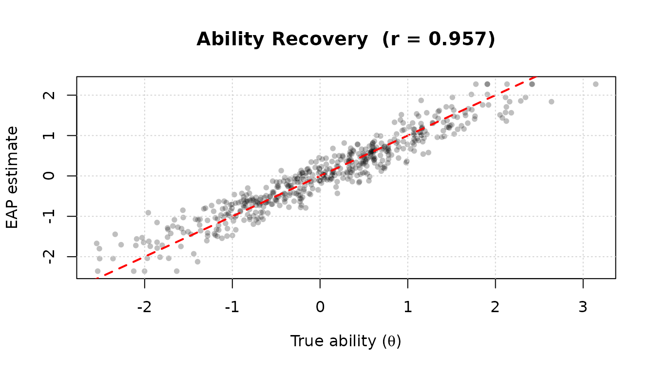

High correlation ( $r > 0.9$ ) between EAP estimates and the true simulated abilities confirms that the item calibration and scoring steps are working correctly.

What’s Next?

Now that you understand irtQ’s item metadata structure and the supported IRT models, you are ready to explore each analysis in depth:

Topic	Vignette	Key Functions
Item parameter estimation	`vignette("item-parameter-estimation")`	`est_irt()`, `est_mg()`, `est_item()`
Ability estimation	`vignette("ability-estimation")`	`est_score()`
Model–data fit	`vignette("model-fit-evaluation")`	`irtfit()`, `sx2_fit()`
DIF detection	`vignette("dif-detection")`	`rdif()`, `grdif()`, `catsib()`
Classification accuracy	`vignette("classification-analysis")`	`cac_lee()`, `cac_rud()`
Utilities	`vignette("utilities")`	`simdat()`, `drm()`, `prm()`, `info()`, `traceline()`, `lwrc()`, `gen.weight()`, `covirt()`
MST panel evaluation	`vignette("mst-panel-evaluation")`	`reval_mst()`

References

Masters, G. N. (1982). A Rasch model for partial credit scoring. Psychometrika, 47(2), 149–174. https://doi.org/10.1007/BF02296272

Muraki, E. (1992). A generalized partial credit model: Application of an EM algorithm. Applied Psychological Measurement, 16(2), 159–176. https://doi.org/10.1177/014662169201600206

Samejima, F. (1969). Estimation of latent ability using a response pattern of graded scores. Psychometrika Monograph Supplement, 34(4, Pt. 2), 1–97. https://doi.org/10.1007/BF03372160