MST Panel Evaluation and Simulation

What is a Multistage-Adaptive Test (MST)?

A Multistage-Adaptive Test (MST) is a computer-based adaptive testing design that sits between fully adaptive Computerized Adaptive Testing (CAT) and traditional linear fixed-form testing. In an MST, the test is divided into stages, each containing one or more pre-assembled groups of items called modules. Routing rules — based on performance on earlier stages — determine which module a test taker receives at each subsequent stage.

The Basic Structure

A typical MST panel is described by its stage-module configuration. For example, a 1-3-3 panel has:

• Stage 1: 1 routing module — everyone starts with the same items
• Stage 2: 3 modules of varying difficulty (e.g., easy, medium, hard)
• Stage 3: 3 modules of varying difficulty (e.g., easy, medium, hard)

The diagram below illustrates the flow of test takers through a 1-3-3 panel (E = Easy, M = Medium, H = Hard):

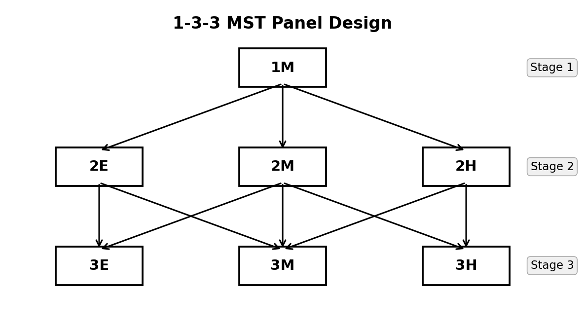
1-3-3 MST panel design. From Stage 1, all examinees begin at module 1M. After Stage 1, they are routed to one of three Stage 2 modules (2E, 2M, 2H) based on their estimated ability. After Stage 2, they are routed to one of three Stage 3 modules (3E, 3M, 3H).

A test taker’s pathway through the MST is the sequence of modules they take, such as 1M → 2E → 3E (for a low-ability examinee) or 1M → 2H → 3H (for a high-ability examinee). In a 1-3-3 panel above, there are 7 such pathways.

Advantages of MST Over Linear Tests and CAT

Feature	Linear	CAT	MST
Adaptivity	None	Item-by-item	Stage-by-stage
Content review	Full review allowed	(Generally) Not allowed	Allowed within module
Item exposure control	Easy	Difficult	Moderate
Test assembly	Pre-assembled	On-the-fly	(Generally) Pre-assembled modules
Operational cost	Low	High	Moderate

MST is especially popular in high-stakes certification and licensure exams because it allows examinees to review and change answers within a module (like a paper test) while still adapting the difficulty level to each examinee.

---

Why Simulate MST Panel Performance?

Designing an operational MST program is rarely a one-shot exercise. Test developers typically draft several candidate panel designs that differ in the number of stages and modules, the difficulty targeting of each module, the routing rule (fixed cut scores vs. an IRT-information-based router such as b-matching or maximum Fisher information), and the scoring method used at each stage. Before committing to one design operationally, they need a way to judge which candidate best serves the purpose of the testing program: a licensure exam may need to maximize precision near the pass/fail cut score, whereas a broad-range achievement test may need uniform precision across the entire ability continuum. Comparing candidate panels against goals like these has long relied on simulating how each design would behave with real examinees (Luecht & Nungester, 1998; Zenisky et al., 2009): generate examinees with known true abilities, route each one through a candidate panel exactly as a real test taker would be routed, and examine how closely the resulting ability estimates recover the true values.

irtQ provides two functions for exactly this purpose. run_mst() simulates a full MST administration — examinee by examinee, stage by stage — and reports the resulting ability estimates and routing pathways. reval_mst() conducts the MST evaluation analytically, via a recursion-based method(Lim et al., 2021), without simulating any individual examinee. This vignette covers both, starting with run_mst(). They describe an MST panel using the same structural inputs, introduced next.

Input Data: The Building Blocks of an MST Panel

run_mst() and reval_mst() describe an MST panel using the same core structural inputs, in addition to the item metadata:

1. Item Bank (x)

A standard irtQ item metadata data frame (see ?shape_df or the Getting Started vignette). Each row describes one item in the item bank. The columns are id, cats, model, par.1, par.2, etc.

2. Module Assignment Matrix (module)

A binary matrix with rows = items (same order as x) and columns = modules. An entry of 1 in row $i$, column $m$ means item $i$ belongs to module $m$.

        M1  M2  M3  M4  M5  M6  M7
item 1 [  1   0   0   0   0   0   0 ]  ← item 1 is in module 1
item 2 [  1   0   0   0   0   0   0 ]
...
item 9 [  0   1   0   0   0   0   0 ]  ← item 9 is in module 2
...

Each item belongs to exactly one module, so each row has exactly one 1 and all other entries are 0.

3. Route Map (route_map)

A binary square matrix of dimension (total modules × total modules). An entry of 1 in row $i$, column $j$ means test takers can be routed from module $i$ directly to module $j$.

For a 1-3-3 panel with 7 modules (M1–M7):

         M1 M2 M3 M4 M5 M6 M7
M1  ──→ [  0  1  1  1  0  0  0 ]   M1 routes to M2, M3, or M4
M2  ──→ [  0  0  0  0  1  1  0 ]   M2 routes to M5 or M6
M3  ──→ [  0  0  0  0  0  1  1 ]   M3 routes to M6 or M7
M4  ──→ [  0  0  0  0  0  1  1 ]   M4 routes to M6 or M7
M5  ──→ [  0  0  0  0  0  0  0 ]   terminal (Stage 3)
M6  ──→ [  0  0  0  0  0  0  0 ]   terminal
M7  ──→ [  0  0  0  0  0  0  0 ]   terminal

Stage 1 modules are identified automatically as those with all-zero columns (no module routes to them). Terminal modules have all-zero rows.

4. Cut Scores (cut_score)

A list of numeric vectors — one element per routing stage transition. Each vector contains the IRT $\theta$ cut points used to determine which next-stage module a test taker receives.

For a 1-3-3 panel with 2 routing stages:

cut_score = list(
  c(-0.5, 0.5),   # Stage 1 → Stage 2: θ̂ < -0.5 → M2 (easy)
                  #                    -0.5 ≤ θ̂ < 0.5 → M3 (medium)
                  #                    θ̂ ≥ 0.5 → M4 (hard)
  c(-0.6, 0.6)    # Stage 2 → Stage 3: θ̂ < -0.6 → easy module
                  #                    -0.6 ≤ θ̂ < 0.6 → medium module
                  #                    θ̂ ≥ 0.6 → hard module
)

cut_score is required by reval_mst(), which always uses inverse-TCC scoring internally, and by run_mst() whenever route_method = NULL. When route_method is instead "bmat" or "mfi", run_mst() ignores cut_score entirely and routes from item difficulty or test information directly, as shown below.

5. True Ability or Observed Responses (theta / response)

reval_mst() always treats theta as a fixed ability grid at which to evaluate bias and CSEM analytically. run_mst() instead uses theta (or response) to simulate individual examinees:

• Supplying theta: a numeric vector of true ability values, one per simulated examinee. run_mst() generates each examinee’s item responses internally from these true values, x, and D.
• Supplying response instead: an already-generated $N \times J$ item response matrix (e.g., from simdat(), or real observed data). theta can still be supplied alongside response, purely for RMSE comparison after the fact — it plays no role in generating the responses themselves.

How theta is constructed changes what the simulation tells you. Drawing it randomly from an assumed population ability distribution — rnorm(1000, 0, 1) in the examples below — evaluates the panel’s overall performance across a single, population-representative batch of examinees, much as a testing program would experience it operationally. Fixing theta at one value and simulating many replications at that single point instead evaluates the panel’s conditional bias and precision at that specific ability level — the same quantity reval_mst() computes analytically, without any simulation. Repeating that single-point simulation across a grid of ability values is exactly the traditional Monte Carlo approach described later in this article, and Example 6 demonstrates it directly with run_mst().

6. Scoring Specification (route_score / final_score)

run_mst() separates the scoring method used for routing decisions at intermediate stages (route_score) from the method used to report each examinee’s final score (final_score). Both arguments take a named list whose method element selects one of irtQ’s ability estimators — "ML", "WL", "MAP", "EAP", "EAP.SUM", or "INV.TCC" — and whose remaining elements supply that estimator’s own arguments, e.g. range for "ML"/"WL", or norm.prior and nquad for "EAP":

route_score = list(method = "EAP", norm.prior = c(0, 1), nquad = 41)
final_score = list(method = "ML", range = c(-4, 4))

Routing and final scoring need not use the same method, and the more principled choice runs this way: "EAP" is usually preferred for routing, because the intermediate ability estimate must always be well-defined, even from a short module. The Stage 1 routing module in particular may have so few items that an examinee answers every one correctly or every one incorrectly — a pattern for which "ML" has no finite solution. "EAP"’s prior keeps the routing estimate finite and stable no matter the response pattern. For the final reported score, "ML" is often preferred instead: by the last stage examinees have answered enough items that such extreme patterns are rare, and "ML" avoids the shrinkage toward the population mean that "EAP"’s prior introduces. "INV.TCC" recovers ability from the observed sum score via the inverse Test Characteristic Curve — the same method reval_mst() uses internally — and is useful when a testing program reports summed scores directly.

The simMST Dataset

irtQ includes simMST, a built-in dataset that packages all four inputs described above. This dataset represents a 1-3-3 MST panel, assembled using module-level target test information functions and design constraints similar to those used in the simulation study of Lim et al. (2021) (it is not the identical dataset from that study), with the following characteristics:

• 7 modules across 3 stages
• 8 items per module across 7 modules (56 unique items total, no item shared across modules)
• All items follow the 3-parameter logistic model (3PLM)
• Item parameters calibrated to span a broad ability range

library(irtQ)

# Inspect the simMST dataset
str(simMST, max.level = 1)
#> List of 5
#>  $ item_bank:'data.frame':   56 obs. of  6 variables:
#>  $ module   : int [1:56, 1:7] 0 0 0 1 0 0 0 0 0 0 ...
#>  $ route_map: int [1:7, 1:7] 0 0 0 0 0 0 0 1 0 0 ...
#>   ..- attr(*, "dimnames")=List of 2
#>  $ cut_score:List of 2
#>  $ theta    : num [1:81] -4 -3.9 -3.8 -3.7 -3.6 -3.5 -3.4 -3.3 -3.2 -3.1 ...

# Item bank: standard irtQ metadata format
head(simMST$item_bank, 10)
#>    id cats model     par.1       par.2      par.3
#> 1   1    2  3PLM 0.8046689  0.88877424 0.07111049
#> 2   2    2  3PLM 1.1698814  1.92935685 0.09127957
#> 3   3    2  3PLM 1.0684706  0.41364009 0.11193439
#> 4   4    2  3PLM 1.2212463  1.53688842 0.07581786
#> 5   5    2  3PLM 1.4571606 -0.75722758 0.06916838
#> 6   6    2  3PLM 1.3195904 -0.82946802 0.05324622
#> 7   7    2  3PLM 0.8683278  0.25561228 0.06429254
#> 8   8    2  3PLM 1.2138528  0.68499259 0.03843348
#> 9   9    2  3PLM 1.2447288  0.05907495 0.12361107
#> 10 10    2  3PLM 1.0414900 -0.42144469 0.08158022

# Module matrix: 56 items × 7 modules
dim(simMST$module)
#> [1] 56  7

# First 16 rows (items 1-16, first 2 modules)
simMST$module[1:16, ]
#>       [,1] [,2] [,3] [,4] [,5] [,6] [,7]
#>  [1,]    0    0    0    1    0    0    0
#>  [2,]    0    0    0    1    0    0    0
#>  [3,]    0    0    0    0    0    0    1
#>  [4,]    1    0    0    0    0    0    0
#>  [5,]    0    1    0    0    0    0    0
#>  [6,]    0    0    0    0    1    0    0
#>  [7,]    0    0    0    1    0    0    0
#>  [8,]    0    0    0    0    0    0    1
#>  [9,]    0    0    0    0    0    1    0
#> [10,]    0    0    0    0    0    1    0
#> [11,]    0    0    0    0    0    0    1
#> [12,]    0    0    0    0    0    1    0
#> [13,]    0    0    1    0    0    0    0
#> [14,]    0    0    0    0    1    0    0
#> [15,]    0    0    1    0    0    0    0
#> [16,]    0    0    0    0    1    0    0

# Route map: 7 × 7 transition matrix
simMST$route_map
#>      V1 V2 V3 V4 V5 V6 V7
#> [1,]  0  1  1  1  0  0  0
#> [2,]  0  0  0  0  1  1  0
#> [3,]  0  0  0  0  1  1  1
#> [4,]  0  0  0  0  0  1  1
#> [5,]  0  0  0  0  0  0  0
#> [6,]  0  0  0  0  0  0  0
#> [7,]  0  0  0  0  0  0  0

The route_map shows:

• Row 1 (Module 1, Stage 1): routes to columns 2, 3, 4 — the three Stage 2 modules
• Rows 2–4 (Modules 2–4, Stage 2): each routes to two or three Stage 3 modules
• Rows 5–7 (Modules 5–7, Stage 3): all zeros — terminal modules

# Cut scores: 2 routing transitions for 3 stages
simMST$cut_score
#> $stage.2
#> [1] -0.4450901  0.4588774
#> 
#> $stage.3
#> [1] -0.4170988  0.4531584

# Ability grid for evaluation
length(simMST$theta)
#> [1] 81
range(simMST$theta)
#> [1] -4  4
head(simMST$theta, 10)
#>  [1] -4.0 -3.9 -3.8 -3.7 -3.6 -3.5 -3.4 -3.3 -3.2 -3.1

Simulating an MST Administration with run_mst()

irtQ provides run_mst() to carry out exactly this kind of simulation. Given an item bank, a route_map, a module matrix, and a vector of true abilities (or a pre-generated response matrix), run_mst() simulates the full MST administration for every examinee — stage-by-stage routing and final scoring — and returns the resulting ability estimates together with the module pathway each examinee traveled.

The examples below use the same simMST 1-3-3 panel introduced above: a routing module at Stage 1, followed by three modules of varying difficulty at each of Stages 2 and 3.

run_mst() supports three routing strategies. Two require no fixed cut scores at all: the default, route_method = "bmat", routes each examinee to the reachable module whose mean item difficulty is closest to their current ability estimate, and route_method = "mfi" routes to the reachable module with the highest test information function (TIF) value at their current estimate. The third, cut-score routing (route_method = NULL), compares the current estimate against a fixed set of cut scores. Start with the default, bmat:

# Item bank and panel structure from simMST
x         <- simMST$item_bank
module    <- simMST$module
route_map <- simMST$route_map

# 1,000 simulated examinees with true abilities from N(0, 1)
set.seed(42)
theta_true <- rnorm(1000, mean = 0, sd = 1)

# bmat routing: no cut scores needed
sim_bmat <- run_mst(
  x            = x,
  route_map    = route_map,
  module       = module,
  theta        = theta_true,
  D            = 1.702,
  route_method = "bmat",
  route_score  = list(method = "EAP", norm.prior = c(0, 1), nquad = 41),
  final_score  = list(method = "ML", range = c(-4, 4)),
  se           = TRUE
)
print(sim_bmat)
#> 
#> Call:
#> run_mst(x = x, route_map = route_map, module = module, theta = theta_true, 
#>     D = 1.702, route_method = "bmat", route_score = list(method = "EAP", 
#>         norm.prior = c(0, 1), nquad = 41), final_score = list(method = "ML", 
#>         range = c(-4, 4)), se = TRUE) 
#> 
#> MST Simulation Results
#> ======================================== 
#> 
#> Panel structure:
#>   Stages              : 3
#>   Modules per stage   : 1 - 3 - 3
#>   Valid pathways      : 7
#>   Routing method      : bmat (b-matching)
#> 
#> Number of examinees : 1000
#> 
#> Ability estimation:
#>   Routing method      : EAP
#>   Final method        : ML
#> 
#> Final ability estimates (est.theta):
#>   Mean : -0.018
#>   SD   : 1.110
#>   Min  : -4.000
#>   Max  : 4.000
#> 
#> Estimation accuracy (est.theta - true.theta):
#>   Bias : 0.007
#>   RMSE : 0.328
#> 
#> Module frequency by stage:
#>   Stage 1: Module 1: 1000 (100.0%)
#>   Stage 2: Module 2: 302 (30.2%),  Module 3: 314 (31.4%),  Module 4: 384 (38.4%)
#>   Stage 3: Module 5: 372 (37.2%),  Module 6: 262 (26.2%),  Module 7: 366 (36.6%)

A closely related alternative is maximum Fisher information (MFI) routing (route_method = "mfi"): instead of comparing mean item difficulty, it routes each examinee to the reachable module that provides the highest TIF value at their current ability estimate.

sim_mfi <- run_mst(
  x            = x,
  route_map    = route_map,
  module       = module,
  theta        = theta_true,
  D            = 1.702,
  route_method = "mfi",
  route_score  = list(method = "EAP", norm.prior = c(0, 1), nquad = 41),
  final_score  = list(method = "ML", range = c(-4, 4)),
  se           = TRUE
)
print(sim_mfi)
#> 
#> Call:
#> run_mst(x = x, route_map = route_map, module = module, theta = theta_true, 
#>     D = 1.702, route_method = "mfi", route_score = list(method = "EAP", 
#>         norm.prior = c(0, 1), nquad = 41), final_score = list(method = "ML", 
#>         range = c(-4, 4)), se = TRUE) 
#> 
#> MST Simulation Results
#> ======================================== 
#> 
#> Panel structure:
#>   Stages              : 3
#>   Modules per stage   : 1 - 3 - 3
#>   Valid pathways      : 7
#>   Routing method      : mfi (Maximum Fisher Information)
#> 
#> Number of examinees : 1000
#> 
#> Ability estimation:
#>   Routing method      : EAP
#>   Final method        : ML
#> 
#> Final ability estimates (est.theta):
#>   Mean : -0.015
#>   SD   : 1.082
#>   Min  : -4.000
#>   Max  : 4.000
#> 
#> Estimation accuracy (est.theta - true.theta):
#>   Bias : 0.011
#>   RMSE : 0.312
#> 
#> Module frequency by stage:
#>   Stage 1: Module 1: 1000 (100.0%)
#>   Stage 2: Module 2: 279 (27.9%),  Module 3: 475 (47.5%),  Module 4: 246 (24.6%)
#>   Stage 3: Module 5: 334 (33.4%),  Module 6: 359 (35.9%),  Module 7: 307 (30.7%)

MFI routing assumes each module’s TIF curve behaves as intended — peaking higher for harder modules as theta increases, and higher for easier modules as theta decreases. In practice this assumption can fail: a harder module’s TIF curve may unexpectedly peak at a low theta value, so that low-ability examinees who should be routed to an easy module instead get routed into the harder one. This is called an anomalous routing, or path reversal, and it is the opposite of what an MST is designed to do.

Alternatively, setting route_method = NULL switches to traditional cut-score routing — the design most commonly used in operational MST programs — where each examinee’s intermediate ability estimate is compared against a fixed set of cut scores to decide the next module:

# Fixed routing cut scores bundled with simMST
cut_score <- simMST$cut_score   # list(c(-0.45, 0.46), c(-0.42, 0.45))

sim_cut <- run_mst(
  x            = x,
  route_map    = route_map,
  module       = module,
  theta        = theta_true,
  D            = 1.702,
  route_method = NULL,
  cut_score    = cut_score,
  route_score  = list(method = "EAP", norm.prior = c(0, 1), nquad = 41),
  final_score  = list(method = "ML", range = c(-4, 4)),
  se           = TRUE
)
print(sim_cut)
#> 
#> Call:
#> run_mst(x = x, route_map = route_map, module = module, theta = theta_true, 
#>     D = 1.702, route_method = NULL, cut_score = cut_score, route_score = list(method = "EAP", 
#>         norm.prior = c(0, 1), nquad = 41), final_score = list(method = "ML", 
#>         range = c(-4, 4)), se = TRUE) 
#> 
#> MST Simulation Results
#> ======================================== 
#> 
#> Panel structure:
#>   Stages              : 3
#>   Modules per stage   : 1 - 3 - 3
#>   Valid pathways      : 7
#>   Routing method      : cut-score based
#> 
#> Number of examinees : 1000
#> 
#> Ability estimation:
#>   Routing method      : EAP
#>   Final method        : ML
#> 
#> Final ability estimates (est.theta):
#>   Mean : -0.009
#>   SD   : 1.102
#>   Min  : -4.000
#>   Max  : 4.000
#> 
#> Estimation accuracy (est.theta - true.theta):
#>   Bias : 0.017
#>   RMSE : 0.331
#> 
#> Module frequency by stage:
#>   Stage 1: Module 1: 1000 (100.0%)
#>   Stage 2: Module 2: 266 (26.6%),  Module 3: 456 (45.6%),  Module 4: 278 (27.8%)
#>   Stage 3: Module 5: 330 (33.0%),  Module 6: 299 (29.9%),  Module 7: 371 (37.1%)

Deriving Principled Cut Scores with find_cut()

Where do cut scores like these come from in the first place? One principled choice is to derive them directly from the modules’ TIF curves themselves: the natural boundary between an easy and a hard module is the theta value at which the hard module’s TIF first overtakes the easy module’s TIF. Below that point the easier module is more informative; above it, the harder module is. This is also exactly the fix for the anomalous-routing problem described above for MFI routing — by fixing the cut point at this proper crossing, low-ability examinees can never be routed into the harder module no matter how its TIF curve behaves at the extremes.

find_cut() automates this search. For every pair of adjacent modules at each stage transition, it scans the theta scale for crossings between the two modules’ TIF curves, keeps only the “proper” crossing (the TIF difference changing sign from negative to positive), and returns the result as a cut_score list that can be passed directly to run_mst().

In fact, the cut scores bundled in simMST$cut_score were generated this same way when the panel was assembled, so recomputing them here should reproduce the same values:

cut_result <- find_cut(
  x         = x,
  module    = module,
  route_map = route_map
)
print(cut_result)
#> MST TIF-Crossing Cut Score Results
#> ==================================================
#> 
#> stage.2
#> -----------------------------------
#>   Modules (index order)    : 2, 3, 4
#>   Modules (difficulty order): 2, 3, 4
#>   Mean item locations      : -0.87, -0.0574, 0.7858
#>   Selected cut score(s)    : -0.4451, 0.4589
#>   Pair details:
#>     [mod2_vs_mod3]
#>       Proper crossing(s)    : 1  [theta = -0.4451]
#>       Anomalous crossing(s) : 1  [theta = 3.3893]  (excluded)
#>       Selected cut score    : -0.4451
#>     [mod3_vs_mod4]
#>       Proper crossing(s)    : 1  [theta = 0.4589]
#>       Selected cut score    : 0.4589
#> 
#> stage.3
#> -----------------------------------
#>   Modules (index order)    : 5, 6, 7
#>   Modules (difficulty order): 5, 6, 7
#>   Mean item locations      : -0.5586, -0.042, 0.5066
#>   Selected cut score(s)    : -0.4171, 0.4532
#>   Pair details:
#>     [mod5_vs_mod6]
#>       Proper crossing(s)    : 1  [theta = -0.4171]
#>       Anomalous crossing(s) : 1  [theta = 1.617]  (excluded)
#>       Selected cut score    : -0.4171
#>     [mod6_vs_mod7]
#>       Proper crossing(s)    : 1  [theta = 0.4532]
#>       Anomalous crossing(s) : 1  [theta = -1.9874]  (excluded)
#>       Selected cut score    : 0.4532
#> ==================================================
#> Usage: run_mst(..., route_method = NULL, cut_score = <result>$cut_score)

# Recomputing reproduces the cut scores already bundled in simMST
cut_result$cut_score
#> $stage.2
#> [1] -0.4450901  0.4588774
#> 
#> $stage.3
#> [1] -0.4170988  0.4531584
simMST$cut_score
#> $stage.2
#> [1] -0.4450901  0.4588774
#> 
#> $stage.3
#> [1] -0.4170988  0.4531584

Calling plot() on the find_cut object visualizes each stage’s module TIF curves, with the selected cut score drawn as a solid vertical line and any excluded anomalous crossings drawn as dashed red lines:

plot(cut_result)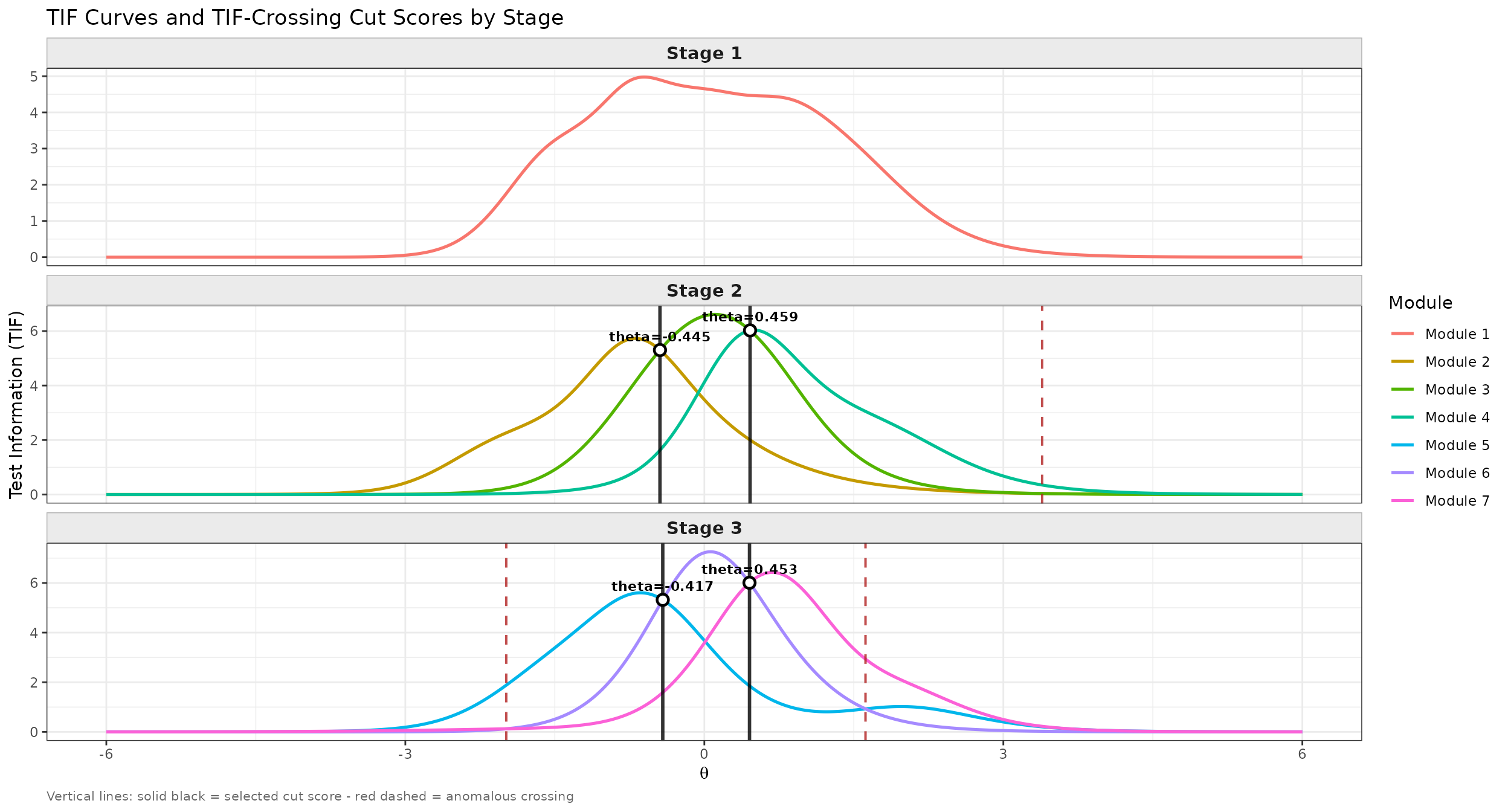

TIF curves for every module in the simMST panel, faceted by stage, with TIF-crossing cut scores from find_cut().

The derived cut scores plug into run_mst() exactly like any other fixed cut scores, by setting route_method = NULL:

sim_findcut <- run_mst(
  x            = x,
  route_map    = route_map,
  module       = module,
  theta        = theta_true,
  D            = 1.702,
  route_method = NULL,
  cut_score    = cut_result$cut_score,
  route_score  = list(method = "EAP", norm.prior = c(0, 1), nquad = 41),
  final_score  = list(method = "ML", range = c(-4, 4)),
  se           = TRUE
)
print(sim_findcut)
#> 
#> Call:
#> run_mst(x = x, route_map = route_map, module = module, theta = theta_true, 
#>     D = 1.702, route_method = NULL, cut_score = cut_result$cut_score, 
#>     route_score = list(method = "EAP", norm.prior = c(0, 1), 
#>         nquad = 41), final_score = list(method = "ML", range = c(-4, 
#>         4)), se = TRUE) 
#> 
#> MST Simulation Results
#> ======================================== 
#> 
#> Panel structure:
#>   Stages              : 3
#>   Modules per stage   : 1 - 3 - 3
#>   Valid pathways      : 7
#>   Routing method      : cut-score based
#> 
#> Number of examinees : 1000
#> 
#> Ability estimation:
#>   Routing method      : EAP
#>   Final method        : ML
#> 
#> Final ability estimates (est.theta):
#>   Mean : -0.010
#>   SD   : 1.080
#>   Min  : -4.000
#>   Max  : 4.000
#> 
#> Estimation accuracy (est.theta - true.theta):
#>   Bias : 0.016
#>   RMSE : 0.323
#> 
#> Module frequency by stage:
#>   Stage 1: Module 1: 1000 (100.0%)
#>   Stage 2: Module 2: 278 (27.8%),  Module 3: 453 (45.3%),  Module 4: 269 (26.9%)
#>   Stage 3: Module 5: 337 (33.7%),  Module 6: 299 (29.9%),  Module 7: 364 (36.4%)

Comparing Routing Methods on Identical Responses with response

All of the calls above let run_mst() simulate item responses internally from theta. When the goal is to compare two routing or scoring strategies fairly, simulation noise in the responses themselves should not be allowed to confound the comparison. Generating the response matrix once with simdat() and feeding it through the response argument removes that source of noise — and is also how run_mst() would be used with real, already-observed response data:

# Generate one response matrix from a fresh set of true abilities
set.seed(123)
theta_true2 <- rnorm(500, mean = 0, sd = 1)
resp_matrix <- simdat(x = x, theta = theta_true2, D = 1.702)
# resp_matrix is an N x J matrix (N examinees x J total items in the bank)

# bmat routing on the pre-generated responses
result_A <- run_mst(
  x            = x,
  route_map    = route_map,
  module       = module,
  theta        = theta_true2,    # kept only for RMSE evaluation below
  response     = resp_matrix,    # pre-generated N x J response matrix
  D            = 1.702,
  route_method = "bmat",
  route_score  = list(method = "EAP", norm.prior = c(0, 1), nquad = 41),
  final_score  = list(method = "ML", range = c(-4, 4)),
  se           = FALSE
)

# find_cut()-based cut-score routing on the SAME responses
result_B <- run_mst(
  x            = x,
  route_map    = route_map,
  module       = module,
  theta        = theta_true2,
  response     = resp_matrix,    # identical responses -> fair comparison
  D            = 1.702,
  route_method = NULL,
  cut_score    = cut_result$cut_score,
  route_score  = list(method = "EAP", norm.prior = c(0, 1), nquad = 41),
  final_score  = list(method = "ML", range = c(-4, 4)),
  se           = FALSE
)

# Any RMSE difference now reflects the routing rule alone, not response noise
rmse_A <- sqrt(mean((result_A$est.theta - theta_true2)^2))
rmse_B <- sqrt(mean((result_B$est.theta - theta_true2)^2))
cat(sprintf("RMSE (bmat):                 %.4f\n", rmse_A))
#> RMSE (bmat):                 0.3119
cat(sprintf("RMSE (find_cut cut scores):  %.4f\n", rmse_B))
#> RMSE (find_cut cut scores):  0.3083

All five calls above return the same kind of result regardless of the routing rule or input format used: a final ability estimate (est.theta), its standard error (se.theta), and the module pathway taken by each examinee (path).

Inspecting the run_mst() Output

print() reports only aggregated information — the panel structure, the routing and final scoring methods, summary statistics (mean, SD, min, max) of the final estimates, and, when true abilities are supplied, overall bias and RMSE. Every examinee’s individual results live in named components of the returned object itself:

# Final ability estimate and its standard error, one value per examinee
head(sim_bmat$est.theta)
#> [1]  1.25259186 -0.58316775  0.63574972  0.56422861  0.15408580  0.02297489
head(sim_bmat$se.theta)
#> [1] 0.2878269 0.2562197 0.2443803 0.2442056 0.2439128 0.2587183

# Routing and final estimates at every stage: an N x n.stage matrix
head(sim_bmat$theta.route)
#>         stage.1     stage.2     stage.3
#> [1,]  0.8423104  1.58893679  1.25259186
#> [2,] -0.4208651 -0.47810582 -0.58316775
#> [3,]  0.3826359  0.54173172  0.63574972
#> [4,]  0.3826359  0.60844003  0.56422861
#> [5,]  0.3826359  0.06174652  0.15408580
#> [6,] -0.0606256  0.31115075  0.02297489

# Module index administered at every stage: an N x n.stage matrix
head(sim_bmat$path)
#>      stage.1 stage.2 stage.3
#> [1,]       1       4       7
#> [2,]       1       3       5
#> [3,]       1       4       7
#> [4,]       1       4       7
#> [5,]       1       4       6
#> [6,]       1       3       7

se.theta in particular never appears in print() output, so accessing it directly is the only way to see how estimation precision varies across examinees — for example, by the Stage 3 (final) module each examinee landed in:

# Mean standard error by terminal (Stage 3) module
tapply(sim_bmat$se.theta, sim_bmat$path[, ncol(sim_bmat$path)], mean)
#>         5         6         7 
#> 2.1794982 0.2469682 3.0071373

The full list of return components — including panel (reused from panel_info()), true.theta, and full.resp (the complete item-level response matrix, populated only when return_full_resp = TRUE) — is summarized in the Function Reference section near the end of this article.

All five calls above drew theta_true (or theta_true2) from a single population distribution, $N(0, 1)$ — appropriate for an overall, population-representative look at how the panel performs across a realistic mix of examinees, the way a testing program would experience it operationally. The complementary question — how the panel performs conditionally, at one specific ability level — requires fixing $\theta$ instead of sampling it, and repeating the simulation many times at that single point. Doing this across a whole grid of ability levels is exactly the traditional approach described next.

---

The Challenge of Evaluating MST Panels

Before deploying an MST panel operationally, test developers need to evaluate its measurement quality: how accurately and precisely does the panel estimate examinee ability at each level of the latent trait $\theta$?

The two key evaluation metrics are:

• Conditional Bias: The average difference between the ability estimate $\hat{\theta}$ and the true ability $\theta$, evaluated at each $\theta$ level. Ideally, bias should be near zero across the full ability range.
• Conditional Standard Error of Measurement (CSEM): The standard deviation of ability estimates at each $\theta$ level. Lower CSEM means more precise measurement.

The Traditional Approach: Monte Carlo Simulation

Conditional evaluation via simulation means repeating the run_mst() procedure shown above systematically across a fixed grid of ability levels, with many replications at each grid point:

1. Fix a set of true ability levels $\theta_1, \theta_2, \ldots$
2. For each $\theta_k$, generate thousands of simulated response patterns
3. Route each simulated examinee through the panel — exactly as run_mst() does above — using the chosen routing rule (cut scores, b-matching, or maximum information)
4. Estimate ability from each simulated response and compute the mean and variance of the estimates
5. Bias = mean($\hat\theta$) − $\theta_k$, CSEM = $\sqrt{\text{Var}(\hat\theta)}$

run_mst() already automates Steps 2–4 for a single $\theta_k$ and a single batch of replications; a full evaluation just wraps it in a loop over the ability grid with a sufficiently large number of replications per grid point (Example 6 below demonstrates exactly this). This approach is conceptually simple, but looping run_mst() this way inherits several practical drawbacks:

• Computationally inefficient: Thousands of response patterns must be generated and scored
• Stochastic: Results fluctuate across simulation replications
• Time-consuming: Evaluating many panel designs or cut score configurations requires many separate simulation runs

The Recursion-Based Analytical Approach: reval_mst()

Lim et al. (2021) proposed a fundamentally different approach: instead of simulating individual examinees, the method directly computes the exact probability distribution of every possible observed score at every stage and pathway using a recursive algorithm.

The key insight is that the conditional distribution of the observed sum score along any pathway can be built up stage by stage using the Lord–Wingersky recursion (Lord & Wingersky, 1984). Given the conditional score distribution of the modules visited so far, the joint distribution at the next stage can be computed exactly — without any random sampling.

Here is the core logic of the recursion:

1. Stage 1: Compute $P(X_1 = x \mid \theta)$ for the routing module using the Lord–Wingersky recursion, where $X_1$ is the total score on Stage 1.

2. Routing: For each possible score $x$ on Stage 1, determine which Stage 2 module a test taker would be routed to (using the cut scores). This converts the score distribution into a pathway probability.

3. Stage 2: For each Stage 2 pathway, compute the joint distribution $P(X_1 + X_2 = s \mid \theta, \text{path})$ by convolving the Stage 1 score distribution with the conditional distribution of the assigned Stage 2 module.

4. Continue recursively through all stages.

5. Ability estimation: Convert each possible final sum score to a $\hat\theta$ estimate using the inverse Test Characteristic Curve (TCC) method — the method implied by IRT-based summed scoring.

   Note on linear interpolation (intpol): When items have non-zero guessing parameters (e.g., 3PLM), the minimum achievable expected sum score exceeds zero — meaning no valid $\hat\theta$ exists for very low observed scores (those below the sum of guessing parameters). With intpol = TRUE (the default), the inverse TCC method applies linear interpolation between the point $(\theta_{\min},\, 0)$ and the lowest TCC-reachable score point, so that every possible sum score receives a valid ability estimate rather than NA.

6. Evaluate: Compute the conditional mean and variance of $\hat\theta$ given the true $\theta$, and derive conditional bias and CSEM.

This method is:

• Exact: The probability distributions are computed analytically, not approximated by random sampling
• Fast: Computation takes seconds, not minutes or hours
• Deterministic: Results are reproducible without any simulation noise
• Comprehensive: Any panel design, cut score configuration, or ability grid can be evaluated in a single function call

The reval_mst() function in irtQ implements this recursion-based method, computing the same conditional bias and CSEM that the Monte Carlo loop above estimates by simulation — but analytically, in a single function call and without any simulation noise.

---

Example 1: Evaluating the simMST Panel

With all inputs in place, running reval_mst() is straightforward:

# Extract components from simMST
x         <- simMST$item_bank
module    <- simMST$module
route_map <- simMST$route_map
cut_score <- simMST$cut_score
theta     <- simMST$theta

# Evaluate the 1-3-3 MST panel
eval_result <- reval_mst(
  x          = x,
  D          = 1.702,
  route_map  = route_map,
  module     = module,
  cut_score  = cut_score,
  theta      = theta,
  range.tcc  = c(-7, 7)
)

The function returns a named list with 7 components. The most important is eval.tb, the evaluation summary table:

# Evaluation table: theta, mu, sigma2, bias, csem
print(eval_result$eval.tb)
#>    theta           mu     sigma2         bias      csem
#> 1   -4.0 -4.808121816 3.42224454 -0.808121816 1.8499310
#> 2   -3.9 -4.789018117 3.43809047 -0.889018117 1.8542089
#> 3   -3.8 -4.766227061 3.45633941 -0.966227061 1.8591233
#> 4   -3.7 -4.739003828 3.47720522 -1.039003828 1.8647266
#> 5   -3.6 -4.706457625 3.50082146 -1.106457625 1.8710482
#> 6   -3.5 -4.667529927 3.52716739 -1.167529927 1.8780754
#> 7   -3.4 -4.620974273 3.55595499 -1.220974273 1.8857240
#> 8   -3.3 -4.565341408 3.58646261 -1.265341408 1.8937958
#> 9   -3.2 -4.498975738 3.61729989 -1.298975738 1.9019201
#> 10  -3.1 -4.420032009 3.64609197 -1.320032009 1.9094743
#> 11  -3.0 -4.326524655 3.66908363 -1.326524655 1.9154852
#> 12  -2.9 -4.216425518 3.68069437 -1.316425518 1.9185136
#> 13  -2.8 -4.087827617 3.67311048 -1.287827617 1.9165361
#> 14  -2.7 -3.939190341 3.63608699 -1.239190341 1.9068526
#> 15  -2.6 -3.769671645 3.55723963 -1.169671645 1.8860646
#> 16  -2.5 -3.579531039 3.42319361 -1.079531039 1.8501875
#> 17  -2.4 -3.370550870 3.22192852 -0.970550870 1.7949731
#> 18  -2.3 -3.146374631 2.94638073 -0.846374631 1.7165025
#> 19  -2.2 -2.912612919 2.59873030 -0.712612919 1.6120578
#> 20  -2.1 -2.676548271 2.19389663 -0.576548271 1.4811808
#> 21  -2.0 -2.446322106 1.76007533 -0.446322106 1.3266783
#> 22  -1.9 -2.229645390 1.33450055 -0.329645390 1.1552058
#> 23  -1.8 -2.032321625 0.95460517 -0.232321625 0.9770390
#> 24  -1.7 -1.857088754 0.64771766 -0.157088754 0.8048091
#> 25  -1.6 -1.703286390 0.42419405 -0.103286390 0.6513018
#> 26  -1.5 -1.567529547 0.27740271 -0.067529547 0.5266903
#> 27  -1.4 -1.445069807 0.18987969 -0.045069807 0.4357519
#> 28  -1.3 -1.331207524 0.14154025 -0.031207524 0.3762184
#> 29  -1.2 -1.222225352 0.11571234 -0.022225352 0.3401652
#> 30  -1.1 -1.115711117 0.10132976 -0.015711117 0.3183234
#> 31  -1.0 -1.010467372 0.09223884 -0.010467372 0.3037085
#> 32  -0.9 -0.906250276 0.08548769 -0.006250276 0.2923828
#> 33  -0.8 -0.803427274 0.07989210 -0.003427274 0.2826519
#> 34  -0.7 -0.702526078 0.07520746 -0.002526078 0.2742398
#> 35  -0.6 -0.603713902 0.07166265 -0.003713902 0.2676988
#> 36  -0.5 -0.506419973 0.06957502 -0.006419973 0.2637708
#> 37  -0.4 -0.409361950 0.06900157 -0.009361950 0.2626815
#> 38  -0.3 -0.311031582 0.06954823 -0.011031582 0.2637200
#> 39  -0.2 -0.210392034 0.07043473 -0.010392034 0.2653954
#> 40  -0.1 -0.107394541 0.07079722 -0.007394541 0.2660775
#> 41   0.0 -0.003020654 0.07009583 -0.003020654 0.2647562
#> 42   0.1  0.101195029 0.06841021  0.001195029 0.2615535
#> 43   0.2  0.203935849 0.06642380  0.003935849 0.2577282
#> 44   0.3  0.304760735 0.06507124  0.004760735 0.2550906
#> 45   0.4  0.404268069 0.06505829  0.004268069 0.2550653
#> 46   0.5  0.503674818 0.06655934  0.003674818 0.2579910
#> 47   0.6  0.604113025 0.06926578  0.004113025 0.2631839
#> 48   0.7  0.706116775 0.07271246  0.006116775 0.2696525
#> 49   0.8  0.809566254 0.07664014  0.009566254 0.2768396
#> 50   0.9  0.913989404 0.08119260  0.013989404 0.2849431
#> 51   1.0  1.018936817 0.08697665  0.018936817 0.2949180
#> 52   1.1  1.124237650 0.09523922  0.024237650 0.3086085
#> 53   1.2  1.230138950 0.10846069  0.030138950 0.3293337
#> 54   1.3  1.337437576 0.13152988  0.037437576 0.3626705
#> 55   1.4  1.447691648 0.17341863  0.047691648 0.4164356
#> 56   1.5  1.563507131 0.24891023  0.063507131 0.4989090
#> 57   1.6  1.688793130 0.37944575  0.088793130 0.6159917
#> 58   1.7  1.828800578 0.59172170  0.128800578 0.7692345
#> 59   1.8  1.989742189 0.91275843  0.189742189 0.9553839
#> 60   1.9  2.177883977 1.36127926  0.277883977 1.1667387
#> 61   2.0  2.398208325 1.93741933  0.398208325 1.3919121
#> 62   2.1  2.652995666 2.61499495  0.552995666 1.6170946
#> 63   2.2  2.940808726 3.34098096  0.740808726 1.8278350
#> 64   2.3  3.256275361 4.04428294  0.956275361 2.0110403
#> 65   2.4  3.590775050 4.65138229  1.190775050 2.1567064
#> 66   2.5  3.933796614 5.10289537  1.433796614 2.2589589
#> 67   2.6  4.274529547 5.36492913  1.674529547 2.3162317
#> 68   2.7  4.603255939 5.43215059  1.903255939 2.3306974
#> 69   2.8  4.912272678 5.32338528  2.112272678 2.3072463
#> 70   2.9  5.196279204 5.07302346  2.296279204 2.2523373
#> 71   3.0  5.452320839 4.72181852  2.452320839 2.1729746
#> 72   3.1  5.679446946 4.30951268  2.579446946 2.0759366
#> 73   3.2  5.878241351 3.87022633  2.678241351 1.9672891
#> 74   3.3  6.050342862 3.43043317  2.750342862 1.8521429
#> 75   3.4  6.198025435 3.00881210  2.798025435 1.7345928
#> 76   3.5  6.323867445 2.61718809  2.823867445 1.6177726
#> 77   3.6  6.430512839 2.26193109  2.830512839 1.5039718
#> 78   3.7  6.520512752 1.94540173  2.820512752 1.3947766
#> 79   3.8  6.596230710 1.66722536  2.796230710 1.2912108
#> 80   3.9  6.659794430 1.42531046  2.759794430 1.1938637
#> 81   4.0  6.713079533 1.21660661  2.713079533 1.1029989

Each row corresponds to one true ability level $\theta$. The columns are:

Column	Meaning
theta	True ability level
mu	Conditional mean of ability estimates $E[\hat\theta \mid \theta]$
sigma2	Conditional variance of ability estimates $\text{Var}[\hat\theta \mid \theta]$
bias	Conditional bias = $\mu - \theta$
csem	Conditional SEM = $\sqrt{\sigma^2}$

A well-designed panel will show:

• bias values close to zero across the full ability range
• csem values that are relatively small and stable (or slightly U-shaped, higher at the extremes where fewer items provide information)

---

Example 2: Visualizing Bias and CSEM

Plotting the evaluation results provides an intuitive picture of the panel’s measurement quality.

eval_tb <- eval_result$eval.tb

# Side-by-side plots: bias (left) and CSEM (right)
par(mfrow = c(1, 2), mar = c(4.5, 4.5, 3, 1))

# Bias plot
plot(
  eval_tb$theta, eval_tb$bias,
  type = "b", pch = 16, col = "steelblue", lwd = 2,
  xlab = expression(theta),
  ylab = "Conditional Bias",
  main = "Conditional Bias",
  ylim = c(-2.5, 2.5)
)
abline(h = 0, col = "red", lty = 2, lwd = 1.5)
grid()

# CSEM plot
plot(
  eval_tb$theta, eval_tb$csem,
  type = "b", pch = 16, col = "darkorange", lwd = 2,
  xlab = expression(theta),
  ylab = "CSEM",
  main = "Conditional SEM (CSEM)",
  ylim = c(0, max(eval_tb$csem) * 1.2)
)
abline(h = mean(eval_tb$csem), col = "red", lty = 2, lwd = 1.5)
legend("topright", legend = "Mean CSEM", lty = 2, col = "red", lwd = 1.5)
grid()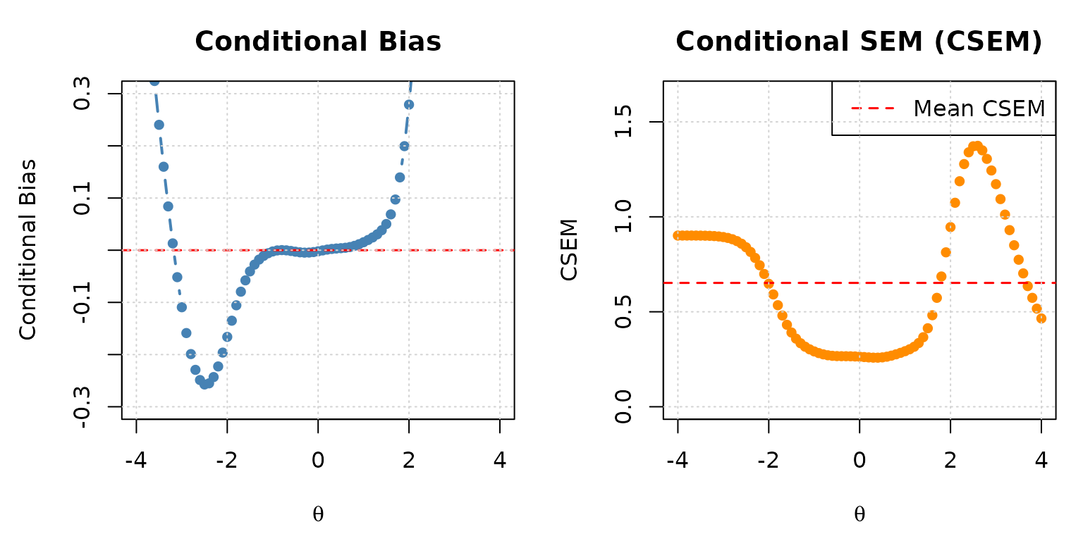

Conditional bias (left) and CSEM (right) for the simMST 1-3-3 panel across the ability scale.

par(mfrow = c(1, 1))

You can also create a combined ggplot2 figure, as shown in the reval_mst() help page:

library(ggplot2)
library(tidyr)
library(dplyr)

eval_tb %>%
  dplyr::select(theta, bias, csem) %>%
  tidyr::pivot_longer(
    cols      = c(bias, csem),
    names_to  = "criterion",
    values_to = "value"
  ) %>%
  ggplot2::ggplot(aes(x = theta, y = value)) +
  ggplot2::geom_hline(yintercept = 0, linetype = "dashed", colour = "grey50") +
  ggplot2::geom_line(aes(colour = criterion, linetype = criterion), linewidth = 1.2) +
  ggplot2::geom_point(aes(shape = criterion), size = 2.5) +
  ggplot2::scale_colour_manual(values = c(bias = "steelblue", csem = "darkorange")) +
  ggplot2::scale_linetype_manual(values = c(bias = "solid", csem = "dashed")) +
  ggplot2::labs(
    x       = expression(theta),
    y       = NULL,
    title   = "1-3-3 MST Panel: Conditional Bias and CSEM",
    colour  = NULL,
    linetype = NULL,
    shape   = NULL
  ) +
  ggplot2::theme_bw() +
  ggplot2::theme(legend.key.width = unit(1.5, "cm"))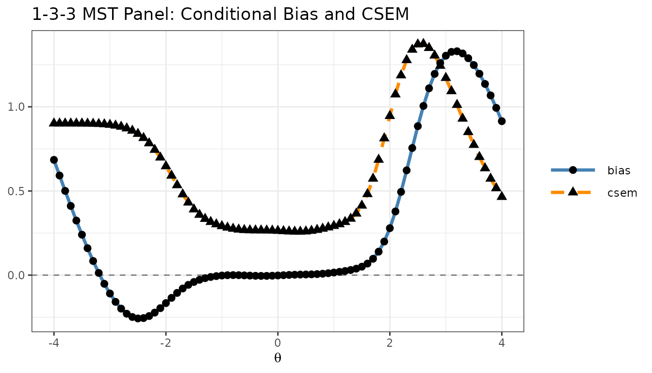

Bias and CSEM plotted together using ggplot2.

---

Example 3: Exploring Other Output Components

Beyond eval.tb, reval_mst() returns intermediate objects that can help diagnose how the panel operates.

Panel Structure (panel.info)

# Panel configuration: which modules belong to each stage
eval_result$panel.info$config
#> $stage.1
#> [1] 1
#> 
#> $stage.2
#> [1] 2 3 4
#> 
#> $stage.3
#> [1] 5 6 7

# All valid pathways through the panel
eval_result$panel.info$pathway
#>        stage.1 stage.2 stage.3
#> path.1       1       2       5
#> path.2       1       2       6
#> path.3       1       3       5
#> path.4       1       3       6
#> path.5       1       3       7
#> path.6       1       4       6
#> path.7       1       4       7

# Number of modules per stage
eval_result$panel.info$n.module
#> stage.1 stage.2 stage.3 
#>       1       3       3

# Total number of stages
eval_result$panel.info$n.stage
#> [1] 3

Items per Module (item.by.mod)

# Item metadata for Module 1 (the routing module)
eval_result$item.by.mod$m.1
#>   id cats model    par.1       par.2      par.3
#> 1  4    2  3PLM 1.221246  1.53688842 0.07581786
#> 2 18    2  3PLM 1.622737  0.06477017 0.05118737
#> 3 19    2  3PLM 1.336215  1.40423576 0.04806838
#> 4 20    2  3PLM 1.629243 -1.55679267 0.08627866
#> 5 29    2  3PLM 2.083387 -0.72116319 0.06071835
#> 6 40    2  3PLM 1.423525 -1.51207055 0.09036353
#> 7 47    2  3PLM 1.749734  0.81776913 0.06977780
#> 8 51    2  3PLM 1.559166 -0.03225149 0.08974932

# Item metadata for Module 5 (Stage 3, first terminal module)
eval_result$item.by.mod$m.5
#>   id cats model     par.1      par.2      par.3
#> 1  6    2  3PLM 1.3195904 -0.8294680 0.05324622
#> 2 14    2  3PLM 1.0655003 -0.7298034 0.07826248
#> 3 16    2  3PLM 1.4237437 -1.6356798 0.06386124
#> 4 21    2  3PLM 1.4501399 -0.5532830 0.15345051
#> 5 26    2  3PLM 1.3768223 -0.7683207 0.11185801
#> 6 28    2  3PLM 1.2187965  1.9922146 0.06489523
#> 7 30    2  3PLM 1.3802801 -0.3492380 0.11699158
#> 8 45    2  3PLM 0.9269771 -1.5949464 0.09669537

Inverse-TCC Ability Estimates (eq.theta)

The eq.theta component contains the IRT $\theta$ estimates corresponding to each possible observed sum score, computed via the inverse TCC method. These are the score-to-$\theta$ mappings used for routing and final ability reporting.

# eq.theta[[stage]][[path]] gives a vector of theta estimates,
# one per possible observed sum score on that partial path

# Stage 1, Path 1 (routing module only — 8 items, scores 0-8)
cat("Theta estimates for Stage 1 (8 items, scores 0-8):\n")
#> Theta estimates for Stage 1 (8 items, scores 0-8):
round(eval_result$eq.theta$stage.1[, 1], 3)
#> [1] -7.000 -2.013 -1.249 -0.676 -0.150  0.373  0.913  1.534  7.000

# Stage 3 has multiple columns — one per complete pathway
cat("Dimensions of eq.theta at Stage 3 (rows = possible scores, cols = pathways):\n")
#> Dimensions of eq.theta at Stage 3 (rows = possible scores, cols = pathways):
dim(eval_result$eq.theta$stage.3)
#> [1] 25  7

The number of rows equals the number of possible sum scores (0 through maximum score) for items along that pathway. Each column corresponds to one complete pathway through the MST.

Inspecting Test Information by Pathway

Comparing item information across pathways reveals why bias and CSEM vary with ability level:

# Retrieve item metadata for the easiest and hardest complete pathways
# (pathway 1 = low ability; last pathway = high ability)
n_paths <- nrow(eval_result$panel.info$pathway)

meta_low  <- eval_result$item.by.path$stage.3$path.1          # low-ability path
meta_high <- eval_result$item.by.path[[3]][[n_paths]]          # high-ability path

theta_grid <- seq(-4, 4, 0.1)

tif_low  <- info(x = meta_low,  theta = theta_grid, D = 1.702)$tif
tif_high <- info(x = meta_high, theta = theta_grid, D = 1.702)$tif

par(mfrow = c(1, 1), mar = c(4.5, 4.5, 3, 1))
plot(
  theta_grid, tif_low,
  type = "l", col = "steelblue", lwd = 2,
  xlab = expression(theta), ylab = "Test Information",
  main = "Test Information: Low-Ability vs. High-Ability Pathway",
  ylim = c(0, max(c(tif_low, tif_high)) * 1.1)
)
lines(theta_grid, tif_high, col = "darkorange", lwd = 2, lty = 2)
legend(
  "topright",
  legend  = c("Low-ability pathway (path 1)", "High-ability pathway (last path)"),
  col     = c("steelblue", "darkorange"),
  lty     = c(1, 2), lwd = 2
)
grid()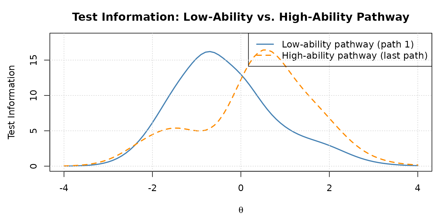

Test information functions for two contrasting pathways in the 1-3-3 panel.

The low-ability pathway peaks at negative $\theta$ values, while the high-ability pathway peaks at positive values — exactly what good MST design achieves.

---

Example 4: Building a Custom MST Panel

To evaluate a panel design from scratch, you need to construct x, module, route_map, and cut_score yourself. This example shows how to do this for a 1-2-2 MST panel with 5 modules and 6 items per module (30 items total).

Design Overview

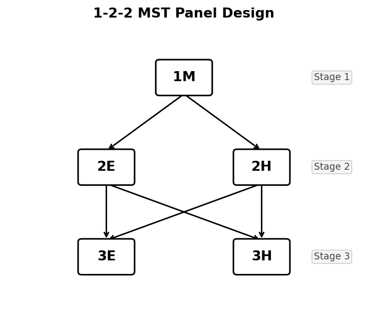
1-2-2 MST panel design. From Stage 1, all examinees begin at module 1M. After Stage 1, they are routed to either 2E (easy) or 2H (hard). After Stage 2, they can be routed to either 3E or 3H regardless of which Stage 2 module they took.

Routing:

• Stage 1 → Stage 2: $\hat\theta < 0$ → M2 (Easy), $\hat\theta \geq 0$ → M3 (Hard)
• Stage 2 → Stage 3: $\hat\theta < 0$ → M4 (Easy), $\hat\theta \geq 0$ → M5 (Hard)

This gives 4 pathways: M1-M2-M4, M1-M2-M5, M1-M3-M4, M1-M3-M5.

Step 1: Build the Item Bank

Items in easy modules have lower difficulty; items in hard modules have higher difficulty. We use the 3PLM for all items.

# 6 items per module × 5 modules = 30 items total
n_per_mod <- 6

# Helper: create item metadata for one module
make_mod_items <- function(a_mean, b_vec, g_val, id_prefix) {
  shape_df(
    par.drm  = list(
      a = rep(a_mean, n_per_mod),
      b = b_vec,
      g = rep(g_val, n_per_mod)
    ),
    item.id  = paste0(id_prefix, 1:n_per_mod),
    cats     = 2,
    model    = "3PLM"
  )
}

# Module 1 (Routing, Stage 1): moderate difficulty
items_m1 <- make_mod_items(
  a_mean   = 1.2,
  b_vec    = c(-0.5, -0.2,  0.0,  0.2,  0.4,  0.6),
  g_val    = 0.15,
  id_prefix = "M1_I"
)

# Module 2 (Easy, Stage 2): lower difficulty
items_m2 <- make_mod_items(
  a_mean   = 1.1,
  b_vec    = c(-2.0, -1.6, -1.3, -1.0, -0.7, -0.4),
  g_val    = 0.15,
  id_prefix = "M2_I"
)

# Module 3 (Hard, Stage 2): higher difficulty
items_m3 <- make_mod_items(
  a_mean   = 1.3,
  b_vec    = c( 0.4,  0.6,  0.9,  1.2,  1.5,  1.8),
  g_val    = 0.15,
  id_prefix = "M3_I"
)

# Module 4 (Easy, Stage 3): lowest difficulty
items_m4 <- make_mod_items(
  a_mean   = 1.0,
  b_vec    = c(-2.5, -2.2, -1.9, -1.6, -1.3, -1.0),
  g_val    = 0.15,
  id_prefix = "M4_I"
)

# Module 5 (Hard, Stage 3): highest difficulty
items_m5 <- make_mod_items(
  a_mean   = 1.4,
  b_vec    = c( 0.8,  1.1,  1.4,  1.7,  2.0,  2.3),
  g_val    = 0.15,
  id_prefix = "M5_I"
)

# Combine into single item bank
item_bank_122 <- dplyr::bind_rows(items_m1, items_m2, items_m3, items_m4, items_m5)
cat("Item bank dimensions:", nrow(item_bank_122), "items ×", ncol(item_bank_122), "columns\n")
#> Item bank dimensions: 30 items × 6 columns
print(item_bank_122)
#>       id cats model par.1 par.2 par.3
#> 1  M1_I1    2  3PLM   1.2  -0.5  0.15
#> 2  M1_I2    2  3PLM   1.2  -0.2  0.15
#> 3  M1_I3    2  3PLM   1.2   0.0  0.15
#> 4  M1_I4    2  3PLM   1.2   0.2  0.15
#> 5  M1_I5    2  3PLM   1.2   0.4  0.15
#> 6  M1_I6    2  3PLM   1.2   0.6  0.15
#> 7  M2_I1    2  3PLM   1.1  -2.0  0.15
#> 8  M2_I2    2  3PLM   1.1  -1.6  0.15
#> 9  M2_I3    2  3PLM   1.1  -1.3  0.15
#> 10 M2_I4    2  3PLM   1.1  -1.0  0.15
#> 11 M2_I5    2  3PLM   1.1  -0.7  0.15
#> 12 M2_I6    2  3PLM   1.1  -0.4  0.15
#> 13 M3_I1    2  3PLM   1.3   0.4  0.15
#> 14 M3_I2    2  3PLM   1.3   0.6  0.15
#> 15 M3_I3    2  3PLM   1.3   0.9  0.15
#> 16 M3_I4    2  3PLM   1.3   1.2  0.15
#> 17 M3_I5    2  3PLM   1.3   1.5  0.15
#> 18 M3_I6    2  3PLM   1.3   1.8  0.15
#> 19 M4_I1    2  3PLM   1.0  -2.5  0.15
#> 20 M4_I2    2  3PLM   1.0  -2.2  0.15
#> 21 M4_I3    2  3PLM   1.0  -1.9  0.15
#> 22 M4_I4    2  3PLM   1.0  -1.6  0.15
#> 23 M4_I5    2  3PLM   1.0  -1.3  0.15
#> 24 M4_I6    2  3PLM   1.0  -1.0  0.15
#> 25 M5_I1    2  3PLM   1.4   0.8  0.15
#> 26 M5_I2    2  3PLM   1.4   1.1  0.15
#> 27 M5_I3    2  3PLM   1.4   1.4  0.15
#> 28 M5_I4    2  3PLM   1.4   1.7  0.15
#> 29 M5_I5    2  3PLM   1.4   2.0  0.15
#> 30 M5_I6    2  3PLM   1.4   2.3  0.15

Step 2: Build the Module Matrix

The module matrix has the same number of rows as item_bank_122 and one column per module. Each row has exactly one 1 — in the column for the module that item belongs to.

n_mods  <- 5
n_items <- nrow(item_bank_122)   # 30

module_122 <- matrix(0L, nrow = n_items, ncol = n_mods)
colnames(module_122) <- paste0("M", 1:n_mods)

# Items 1-6 → M1, items 7-12 → M2, ..., items 25-30 → M5
for (m in 1:n_mods) {
  idx <- ((m - 1) * n_per_mod + 1):(m * n_per_mod)
  module_122[idx, m] <- 1L
}

# Verify: each row sums to 1, each column sums to n_per_mod
cat("Row sums (all should be 1):\n"); print(table(rowSums(module_122)))
#> Row sums (all should be 1):
#> 
#>  1 
#> 30
cat("Column sums (all should be", n_per_mod, "):\n"); print(colSums(module_122))
#> Column sums (all should be 6 ):
#> M1 M2 M3 M4 M5 
#>  6  6  6  6  6

Step 3: Build the Route Map

route_map_122 <- matrix(0L, nrow = n_mods, ncol = n_mods)
rownames(route_map_122) <- colnames(route_map_122) <- paste0("M", 1:n_mods)

# Stage 1 → Stage 2
route_map_122[1, 2] <- 1L   # M1 → M2 (low ability)
route_map_122[1, 3] <- 1L   # M1 → M3 (high ability)

# Stage 2 → Stage 3 (both M2 and M3 can route to either M4 or M5)
route_map_122[2, 4] <- 1L   # M2 → M4
route_map_122[2, 5] <- 1L   # M2 → M5
route_map_122[3, 4] <- 1L   # M3 → M4
route_map_122[3, 5] <- 1L   # M3 → M5

print(route_map_122)
#>    M1 M2 M3 M4 M5
#> M1  0  1  1  0  0
#> M2  0  0  0  1  1
#> M3  0  0  0  1  1
#> M4  0  0  0  0  0
#> M5  0  0  0  0  0

Step 4: Define Cut Scores

# 1 cut point for each of the 2 routing transitions (2-way branching)
cut_score_122 <- list(
  c(0),    # Stage 1 → Stage 2: θ̂ < 0 → M2, θ̂ ≥ 0 → M3
  c(0)     # Stage 2 → Stage 3: θ̂ < 0 → M4, θ̂ ≥ 0 → M5
)

Step 5: Evaluate the Custom Panel

# Evaluation grid: -3 to 3 in steps of 0.5 (coarser for speed)
theta_grid_122 <- seq(-3, 3, 0.5)

eval_122 <- reval_mst(
  x         = item_bank_122,
  D         = 1.702,
  route_map = route_map_122,
  module    = module_122,
  cut_score = cut_score_122,
  theta     = theta_grid_122,
  range.tcc = c(-5, 5)
)

# Evaluation table
print(eval_122$eval.tb)
#>    theta          mu    sigma2         bias      csem
#> 1   -3.0 -3.19623125 0.8592354 -0.196231249 0.9269495
#> 2   -2.5 -2.72861584 0.7871656 -0.228615843 0.8872235
#> 3   -2.0 -2.11902994 0.5155952 -0.119029937 0.7180496
#> 4   -1.5 -1.52846765 0.2785520 -0.028467654 0.5277803
#> 5   -1.0 -0.99289282 0.2024505  0.007107183 0.4499450
#> 6   -0.5 -0.47947559 0.1729555  0.020524412 0.4158792
#> 7    0.0 -0.01380778 0.1486202 -0.013807784 0.3855129
#> 8    0.5  0.46107384 0.1534703 -0.038926159 0.3917529
#> 9    1.0  0.99556805 0.1267071 -0.004431952 0.3559594
#> 10   1.5  1.52787128 0.1395430  0.027871283 0.3735546
#> 11   2.0  2.15212965 0.5041920  0.152129651 0.7100648
#> 12   2.5  3.12555584 1.5165325  0.625555842 1.2314757
#> 13   3.0  4.12958178 1.4429566  1.129581775 1.2012313

eval_tb_122 <- eval_122$eval.tb

par(mfrow = c(1, 2), mar = c(4.5, 4.5, 3, 1))

plot(
  eval_tb_122$theta, eval_tb_122$bias,
  type = "b", pch = 16, col = "steelblue", lwd = 2,
  xlab = expression(theta), ylab = "Conditional Bias",
  main = "1-2-2 Panel: Conditional Bias",
  ylim = range(c(-0.4, 0.4, eval_tb_122$bias))
)
abline(h = 0, col = "red", lty = 2, lwd = 1.5)
grid()

plot(
  eval_tb_122$theta, eval_tb_122$csem,
  type = "b", pch = 16, col = "darkorange", lwd = 2,
  xlab = expression(theta), ylab = "CSEM",
  main = "1-2-2 Panel: CSEM",
  ylim = c(0, max(eval_tb_122$csem) * 1.2)
)
grid()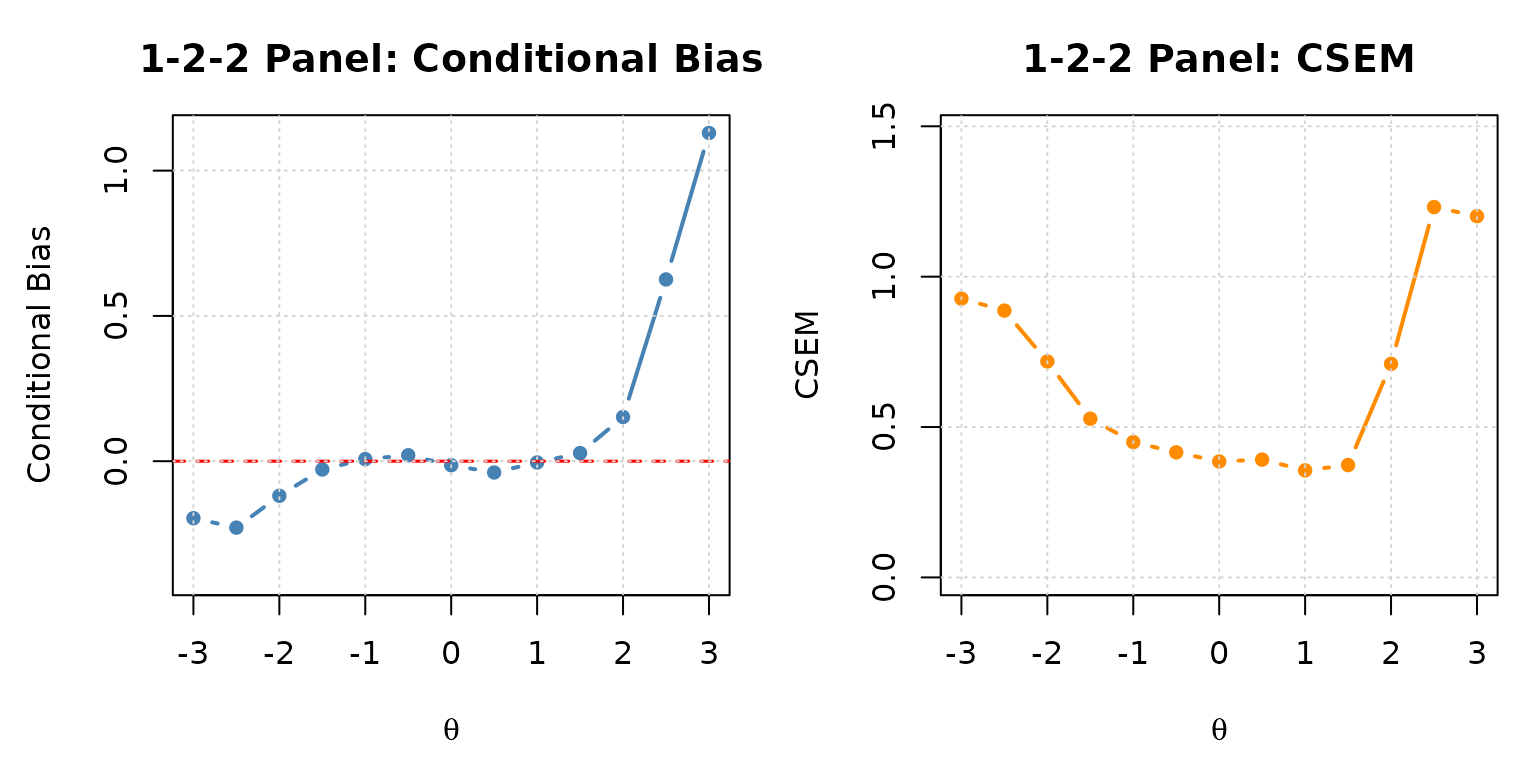

Conditional bias and CSEM for the custom 1-2-2 MST panel.

par(mfrow = c(1, 1))

Step 6: Inspect the Panel Pathways

# Confirmed pathways through the 1-2-2 panel
eval_122$panel.info$pathway
#>        stage.1 stage.2 stage.3
#> path.1       1       2       4
#> path.2       1       2       5
#> path.3       1       3       4
#> path.4       1       3       5

The 1-2-2 panel has 4 pathways — considerably fewer than the 1-3-3 panel’s 7 pathways. The simpler branching structure is appropriate for smaller-scale tests or when fewer stage-3 difficulty levels are needed.

---

Example 5: Comparing Two Cut Score Configurations

Cut score placement directly affects measurement bias. Placing cuts too close to the centre can cause mid-ability examinees to be routed sub-optimally. Here we compare the original c(-0.5, 0.5) cut scores with a wider configuration c(-1.0, 1.0) for the 1-3-3 panel.

# Alternative cut scores: wider routing bands
cut_score_wide <- list(c(-1.0, 1.0), c(-1.0, 1.0))

eval_wide <- reval_mst(
  x         = x,
  D         = 1.702,
  route_map = route_map,
  module    = module,
  cut_score = cut_score_wide,
  theta     = theta,
  range.tcc = c(-7, 7)
)

tb_orig <- eval_result$eval.tb
tb_wide <- eval_wide$eval.tb

par(mfrow = c(1, 2), mar = c(4.5, 4.5, 3, 1))

# Bias comparison
ylim_bias <- range(c(tb_orig$bias, tb_wide$bias, -0.4, 0.4))
plot(
  tb_orig$theta, tb_orig$bias,
  type = "b", pch = 16, col = "steelblue", lwd = 2,
  xlab = expression(theta), ylab = "Conditional Bias",
  main = "Bias Comparison", ylim = ylim_bias
)
lines(tb_wide$theta, tb_wide$bias,
      type = "b", pch = 17, col = "darkorange", lwd = 2, lty = 2)
abline(h = 0, col = "grey50", lty = 3)
legend("topright",
       legend = c("Original cuts (±0.5)", "Wider cuts (±1.0)"),
       col    = c("steelblue", "darkorange"),
       pch    = c(16, 17), lty = c(1, 2), lwd = 2, cex = 0.85)
grid()

# CSEM comparison
ylim_csem <- c(0, max(c(tb_orig$csem, tb_wide$csem)) * 1.2)
plot(
  tb_orig$theta, tb_orig$csem,
  type = "b", pch = 16, col = "steelblue", lwd = 2,
  xlab = expression(theta), ylab = "CSEM",
  main = "CSEM Comparison", ylim = ylim_csem
)
lines(tb_wide$theta, tb_wide$csem,
      type = "b", pch = 17, col = "darkorange", lwd = 2, lty = 2)
legend("topright",
       legend = c("Original cuts (±0.5)", "Wider cuts (±1.0)"),
       col    = c("steelblue", "darkorange"),
       pch    = c(16, 17), lty = c(1, 2), lwd = 2, cex = 0.85)
grid()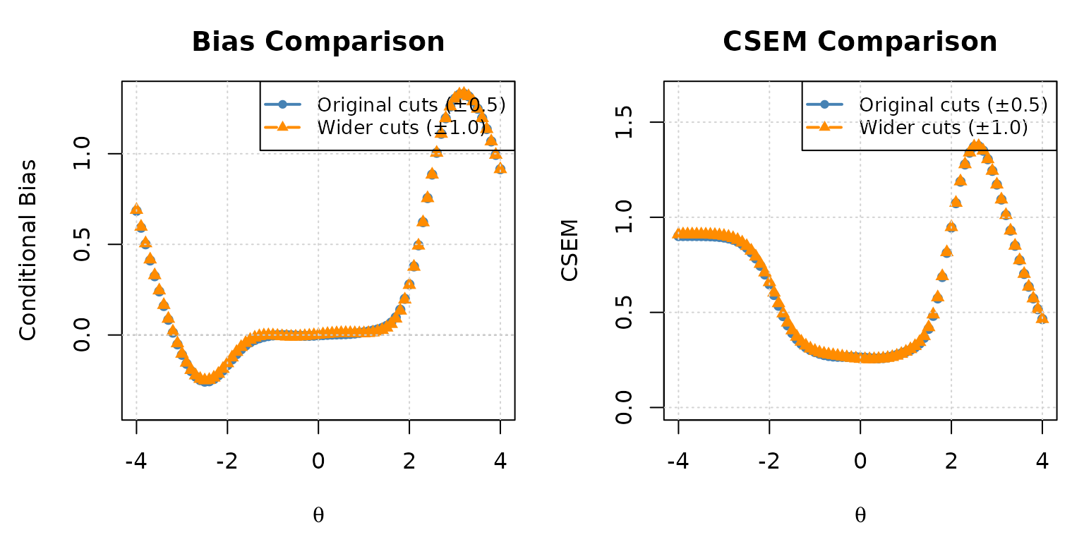

CSEM comparison: original vs. wider cut scores in the 1-3-3 panel.

par(mfrow = c(1, 1))

Wide cuts concentrate test takers in the middle module of Stage 2 and 3 for the most ability levels, which tends to reduce bias near the centre but may increase CSEM at the ability extremes.

---

Example 6: Validating reval_mst() Against a run_mst() Monte Carlo Simulation

The “Why Simulate MST Panel Performance?” section introduced run_mst() and noted that turning a single simulation run into a full panel evaluation means looping it over a $\theta$ grid with many replications per point — the traditional Monte Carlo approach. Lim et al. (2021) validated their recursion-based analytical method against exactly this kind of simulation, and the closeness of the agreement they found depended on the scoring method used. When the simulation used the same scoring the recursion assumes throughout — an equated-number-correct (ENC) score, a deterministic score-to-$\theta$ transformation conceptually analogous to reval_mst()’s internal inverse-TCC scoring — the simulated and analytical results matched closely at every $\theta$, and converged further as replications increased. When the simulation instead used a combination more common in practice — EAP for routing, maximum likelihood (MLE) for the final score — the two methods still agreed closely in the central ability range, but diverged toward the extremes, where the item pool carries little information and MLE behaves quite differently from the inverse-TCC-based recursion. That region of close central agreement widens as test length increases.

We reproduce that second condition directly here for the simMST panel, using the same scoring combination Lim et al. (2021) used in their own validation: route_score = "EAP" for routing at each interim stage, and final_score = "ML" for the reported final score. Neither method matches reval_mst()’s internal inverse-TCC logic, so the two results are not expected to coincide everywhere; the comparison below should reproduce the same central-agreement-with-tail-divergence pattern Lim et al. (2021) reported.

Because the exact values stored in simMST$theta are not needed for this comparison, we define our own explicit evaluation grid so that the Monte Carlo simulation and the analytical computation are guaranteed to line up point-for-point:

# An explicit, independent evaluation grid
theta_grid <- seq(-5, 5, 0.5)
n_reps     <- 300   # simulated examinees per grid point

# Repeat each grid point n_reps times into one long vector of true abilities
set.seed(2026)
true_theta <- rep(theta_grid, each = n_reps)

Step 1 — Monte Carlo simulation with run_mst(). All n_reps replications at every grid point are simulated in a single call by passing the full true_theta vector. Routing uses the panel’s fixed cut scores (matching the routing rule reval_mst() assumes), with EAP routing scores and ML final scores — the scoring combination Lim et al. (2021) used in their own Monte Carlo validation:

sim_mc <- run_mst(
  x            = x,
  route_map    = route_map,
  module       = module,
  theta        = true_theta,
  D            = 1.702,
  route_method = NULL,
  cut_score    = cut_score,
  route_score  = list(method = "EAP", norm.prior = c(0, 1), nquad = 41),
  final_score  = list(method = "ML", range = c(-4, 4)),
  se           = FALSE,
  verbose      = FALSE
)

# Empirical bias and RMSE at each grid point
mc_tb <- data.frame(theta = true_theta, est.theta = sim_mc$est.theta)
diff_mc  <- mc_tb$est.theta - mc_tb$theta
bias_mc  <- tapply(diff_mc, mc_tb$theta, mean)
rmse_mc  <- tapply(diff_mc, mc_tb$theta, function(d) sqrt(mean(d^2)))

mc_result <- data.frame(
  theta = as.numeric(names(bias_mc)),
  bias  = as.numeric(bias_mc),
  rmse  = as.numeric(rmse_mc)
)
mc_result <- mc_result[order(mc_result$theta), ]

Step 2 — Analytical computation with reval_mst() on the same theta_grid, so the comparison is point-for-point:

eval_grid <- reval_mst(
  x         = x,
  D         = 1.702,
  route_map = route_map,
  module    = module,
  cut_score = cut_score,
  theta     = theta_grid,
  range.tcc = c(-7, 7)
)

tb_grid      <- eval_grid$eval.tb
tb_grid$rmse <- sqrt(tb_grid$sigma2 + tb_grid$bias^2)

Step 3 — Overlay the two results:

par(mfrow = c(1, 2), mar = c(4.5, 4.5, 3, 1))

# Bias: Monte Carlo (points) vs. analytical (line)
plot(
  tb_grid$theta, tb_grid$bias,
  type = "l", lwd = 2, col = "steelblue",
  xlab = expression(theta), ylab = "Bias", main = "Bias: Simulation vs. Analytical",
  ylim = range(c(tb_grid$bias, mc_result$bias, -0.3, 0.3))
)
points(mc_result$theta, mc_result$bias, pch = 16, col = "darkorange")
abline(h = 0, col = "grey50", lty = 3)
legend("topright",
       legend = c("reval_mst() (analytical)", "run_mst() (Monte Carlo)"),
       col = c("steelblue", "darkorange"), lty = c(1, NA), pch = c(NA, 16),
       lwd = c(2, NA), cex = 0.8)
grid()

# RMSE: Monte Carlo (points) vs. analytical (line)
plot(
  tb_grid$theta, tb_grid$rmse,
  type = "l", lwd = 2, col = "steelblue",
  xlab = expression(theta), ylab = "RMSE", main = "RMSE: Simulation vs. Analytical",
  ylim = c(0, max(c(tb_grid$rmse, mc_result$rmse)) * 1.2)
)
points(mc_result$theta, mc_result$rmse, pch = 16, col = "darkorange")
legend("topright",
       legend = c("reval_mst() (analytical)", "run_mst() (Monte Carlo)"),
       col = c("steelblue", "darkorange"), lty = c(1, NA), pch = c(NA, 16),
       lwd = c(2, NA), cex = 0.8)
grid()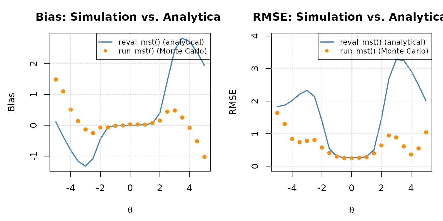

Empirical bias and RMSE from a run_mst() Monte Carlo simulation (points) overlaid on the analytical reval_mst() curve (line).

par(mfrow = c(1, 1))

In the central ability range — which Lim et al. (2021) reported as roughly $-1.5 \le \theta \le 1.5$ for this scoring combination, widening for longer tests — the Monte Carlo points should track the analytical curve closely, with the small remaining deviations attributable to sampling error at n_reps = 300 replications per grid point (these shrink further as n_reps increases). Toward the extremes, the two are expected to diverge: both EAP routing and ML final scoring depart from reval_mst()’s internal inverse-TCC logic, and that departure grows where the item pool carries little information and EAP/MLE estimates behave quite differently from the inverse-TCC-based recursion. This mirrors the pattern Lim et al. (2021) reported for this identical EAP-routing/MLE-final condition. Matching the recursion’s own scoring exactly — route_score = "INV.TCC" and final_score = "INV.TCC" instead of "EAP"/"ML" — would close most of this gap. reval_mst() is therefore best read as predicting the performance of a panel routed and scored via inverse-TCC; whenever a program uses a different scoring approach operationally, a run_mst() simulation like this one remains the more direct check, particularly for ability levels far from the panel’s region of peak information.

Step 4 — Confirm the gap closes under matched scoring. As a final check, re-run the same simulation with route_score = "INV.TCC" and final_score = "INV.TCC", matching reval_mst()’s internal logic exactly:

sim_mc_matched <- run_mst(
  x            = x,
  route_map    = route_map,
  module       = module,
  theta        = true_theta,
  D            = 1.702,
  route_method = NULL,
  cut_score    = cut_score,
  route_score  = list(method = "INV.TCC", range.tcc = c(-7, 7)),
  final_score  = list(method = "INV.TCC", range.tcc = c(-7, 7)),
  se           = FALSE,
  verbose      = FALSE
)

# Empirical bias and RMSE at each grid point, matched-scoring condition
diff_matched <- sim_mc_matched$est.theta - true_theta
bias_matched <- tapply(diff_matched, true_theta, mean)
rmse_matched <- tapply(diff_matched, true_theta, function(d) sqrt(mean(d^2)))

mc_result_matched <- data.frame(
  theta = as.numeric(names(bias_matched)),
  bias  = as.numeric(bias_matched),
  rmse  = as.numeric(rmse_matched)
)
mc_result_matched <- mc_result_matched[order(mc_result_matched$theta), ]

Comparing all three at the tail grid points, where the EAP/ML condition diverged most from the analytical curve:

compare_tb <- data.frame(
  theta              = theta_grid,
  analytical_bias    = round(tb_grid$bias, 3),
  EAP_ML_bias        = round(mc_result$bias, 3),
  INVTCC_INVTCC_bias = round(mc_result_matched$bias, 3),
  analytical_rmse    = round(tb_grid$rmse, 3),
  EAP_ML_rmse        = round(mc_result$rmse, 3),
  INVTCC_INVTCC_rmse = round(mc_result_matched$rmse, 3)
)
compare_tb[compare_tb$theta <= -3 | compare_tb$theta >= 3, ]
#>    theta analytical_bias EAP_ML_bias INVTCC_INVTCC_bias analytical_rmse
#> 1   -5.0           0.108       1.488             -0.017           1.833
#> 2   -4.5          -0.367       1.100             -0.472           1.872
#> 3   -4.0          -0.808       0.509             -0.783           2.019
#> 4   -3.5          -1.168       0.136             -1.160           2.211
#> 5   -3.0          -1.327      -0.134             -1.254           2.330
#> 17   3.0           2.452       0.481              2.494           3.277
#> 18   3.5           2.824       0.252              2.819           3.254
#> 19   4.0           2.713      -0.088              2.741           2.929
#> 20   4.5           2.375      -0.521              2.410           2.488
#> 21   5.0           1.942      -1.023              1.955           2.007
#>    EAP_ML_rmse INVTCC_INVTCC_rmse
#> 1        1.637              1.785
#> 2        1.300              1.868
#> 3        0.836              2.022
#> 4        0.738              2.181
#> 5        0.779              2.262
#> 17       0.883              3.302
#> 18       0.608              3.252
#> 19       0.359              2.938
#> 20       0.546              2.491
#> 21       1.037              2.006

The same comparison, overlaid across the full ability range:

par(mfrow = c(1, 2), mar = c(4.5, 4.5, 3, 1))

# Bias: matched-scoring Monte Carlo (points) vs. analytical (line)
plot(
  tb_grid$theta, tb_grid$bias,
  type = "l", lwd = 2, col = "steelblue",
  xlab = expression(theta), ylab = "Bias",
  main = "Bias: Simulation vs. Analytical",
  ylim = range(c(tb_grid$bias, mc_result_matched$bias, -0.3, 0.3))
)
points(mc_result_matched$theta, mc_result_matched$bias, pch = 16, col = "forestgreen")
abline(h = 0, col = "grey50", lty = 3)
legend("topright",
       legend = c("reval_mst() (analytical)", "run_mst() (INV.TCC/INV.TCC)"),
       col = c("steelblue", "forestgreen"), lty = c(1, NA), pch = c(NA, 16),
       lwd = c(2, NA), cex = 0.8)
grid()

# RMSE: matched-scoring Monte Carlo (points) vs. analytical (line)
plot(
  tb_grid$theta, tb_grid$rmse,
  type = "l", lwd = 2, col = "steelblue",
  xlab = expression(theta), ylab = "RMSE",
  main = "RMSE: Simulation vs. Analytical",
  ylim = c(0, max(c(tb_grid$rmse, mc_result_matched$rmse)) * 1.2)
)
points(mc_result_matched$theta, mc_result_matched$rmse, pch = 16, col = "forestgreen")
legend("topright",
       legend = c("reval_mst() (analytical)", "run_mst() (INV.TCC/INV.TCC)"),
       col = c("steelblue", "forestgreen"), lty = c(1, NA), pch = c(NA, 16),
       lwd = c(2, NA), cex = 0.8)
grid()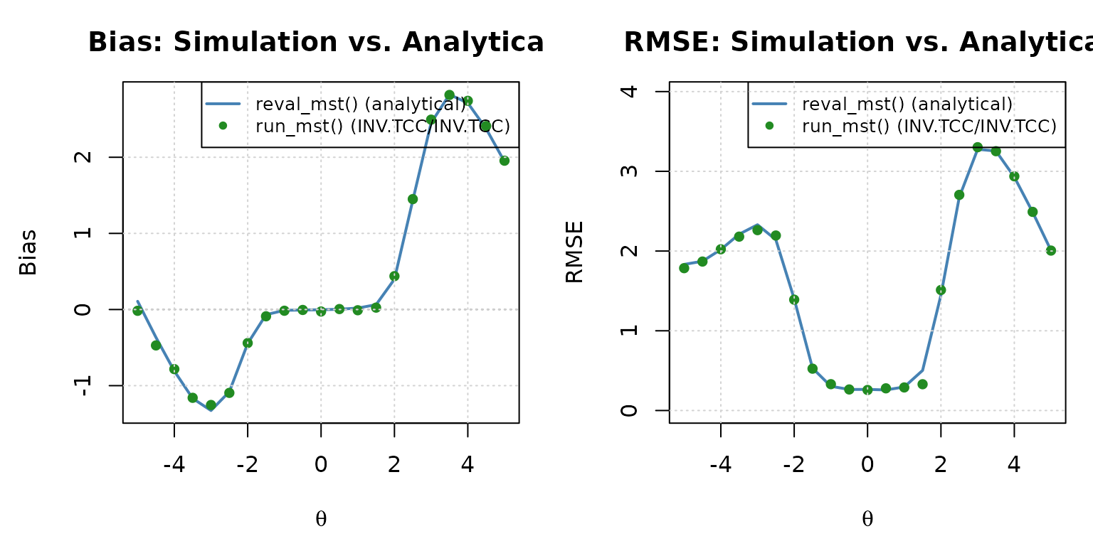

Empirical bias and RMSE from the INV.TCC/INV.TCC run_mst() Monte Carlo simulation (points) overlaid on the analytical reval_mst() curve (line).

par(mfrow = c(1, 1))

Both the table and the plot confirm the same conclusion: the INV.TCC/INV.TCC condition tracks the analytical bias and RMSE closely across the entire ability range, including the extremes where the EAP/ML condition diverged.

---

Function Reference

reval_mst() Arguments

Argument	Type	Default	Description
x	data.frame	—	Item bank metadata (irtQ format)
D	numeric	1	Scaling constant (use 1.702 for normal-ogive approximation)
route_map	matrix	—	Binary square matrix of module transitions
module	matrix	—	Binary matrix mapping items to modules
cut_score	list	—	List of routing cut score vectors (one per stage transition)
theta	numeric	seq(-5, 5, 1)	Ability grid for evaluation
intpol	logical	TRUE	Linear interpolation for out-of-range TCC scores
range.tcc	numeric(2)	c(-7, 7)	Ability range for inverse TCC scoring
tol	numeric	1e-4	Convergence tolerance for bisection in inverse TCC

reval_mst() Return Value

Component	Description
panel.info	Panel structure: $config, $pathway, $n.module, $n.stage
item.by.mod	List of item metadata data frames, one per module
item.by.path	List of cumulative item metadata per stage and pathway
eq.theta	Inverse-TCC $\theta$ estimates for each possible score, by stage and pathway
cdist.by.mod	Conditional score distributions per module, indexed by $\theta$
jdist.by.path	Joint conditional score distributions, indexed by $\theta$ and stage
eval.tb	Evaluation table: theta, mu, sigma2, bias, csem

run_mst() Arguments

Argument	Type	Default	Description
x	data.frame	—	Item bank metadata (irtQ format)
route_map	matrix	—	Binary square matrix of module transitions
module	matrix	—	Binary matrix mapping items to modules
theta	numeric	—	True ability for each simulated examinee (or supply response instead)
response	matrix	NULL	Pre-generated response matrix, used instead of simulating from theta
D	numeric	1	Scaling constant (use 1.702 for normal-ogive approximation)
ini_mod	integer	NULL	Fixed Stage-1 module for all examinees; NULL assigns each independently at random
route_method	character	"bmat"	"bmat", "mfi", or NULL for fixed cut-score routing
cut_score	list	NULL	List of routing cut score vectors; used only when route_method = NULL
route_score	list	—	Scoring method used at intermediate stages (ML, WL, MAP, EAP, EAP.SUM, INV.TCC, …)
final_score	list	—	Scoring method used for the final reported score
se	logical	TRUE	Whether to compute standard errors of the final score
missing	scalar	NA	Value representing a not-administered response in response
verbose	logical	TRUE	Whether to print simulation progress messages to the console
return_full_resp	logical	FALSE	If TRUE, also returns the full N x J item-level response matrix as full.resp

run_mst() Return Value

Component	Description
est.theta	Final ability estimate for each simulated examinee
se.theta	Standard error of the final ability estimate
theta.route	Intermediate ability estimate used for routing at each stage
path	Module pathway taken by each examinee
true.theta	True ability supplied as input (NA when response was supplied instead)
panel	Panel structure information (from panel_info())
full.resp	Full item-level response matrix, if return_full_resp = TRUE

---

References

Lim, H., Davey, T., & Wells, C. S. (2021). A recursion-based analytical approach to evaluate the performance of MST. Journal of Educational Measurement, 58(2), 154–178. https://doi.org/10.1111/jedm.12276

Lord, F. M., & Wingersky, M. S. (1984). Comparison of IRT true-score and equipercentile observed-score equatings. Applied Psychological Measurement, 8(4), 453–461. https://doi.org/10.1177/014662168400800409

Luecht, R. M., & Nungester, R. J. (1998). Some practical examples of computer-adaptive sequential testing. Journal of Educational Measurement, 35(3), 229–249. https://doi.org/10.1111/j.1745-3984.1998.tb00537.x

Zenisky, A., Hambleton, R. K., & Luecht, R. M. (2009). Multistage testing: Issues, designs, and research. In W. J. van der Linden & C. A. W. Glas (Eds.), Elements of adaptive testing (pp. 355–372). Springer. https://doi.org/10.1007/978-0-387-85461-8_18