Plot TIF Curves and Cut Scores from a find_cut Result

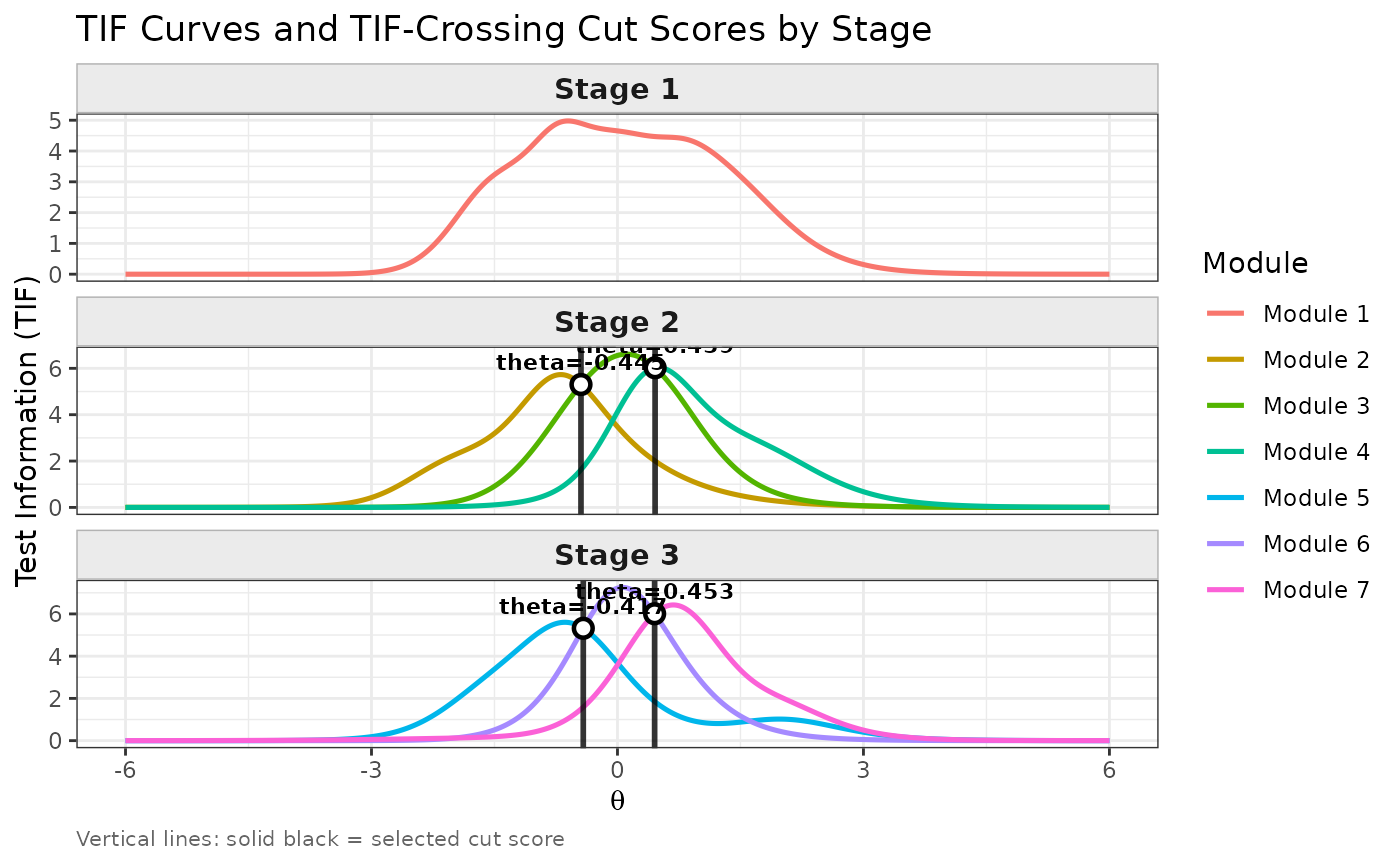
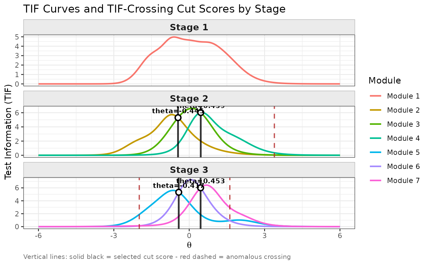
Produces a ggplot2 visualisation of the Test Information Function (TIF) curves for each module, faceted by stage, with vertical lines marking the selected cut scores (proper TIF crossings) and, optionally, any anomalous crossings detected by find_cut.

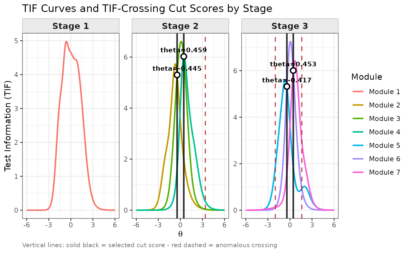
Each stage occupies one panel. Stage 1 (routing module) appears first. Stages with routing decisions show TIF curves for all candidate modules and mark the selected cut score(s) with a solid black vertical line and a theta value label at the crossing point.

Usage

# S3 method for class 'find_cut'
plot(
  x,
  theta_range = NULL,
  show_anomalous = TRUE,
  label_cuts = TRUE,
  layout = c("vertical", "horizontal"),
  ...
)

Arguments

x

An object of class "find_cut" returned by find_cut.

theta_range

A numeric vector of length 2 specifying the theta range shown on the x-axis. Defaults to the full range stored in x$tif_data.

show_anomalous

Logical. If TRUE (default), anomalous TIF crossings (negative-slope crossings excluded from the cut scores) are shown as dashed red vertical lines.

label_cuts

Logical. If TRUE (default), each selected cut score is annotated with its theta value above the crossing point.

layout

Character string controlling the panel arrangement. "vertical" (default) stacks each stage in its own row (one column of panels, stage 1 at the top). "horizontal" places each stage in its own column (one row of panels, stage 1 at the left).

...

Currently unused. Reserved for future arguments.

Value

A ggplot object. The object is printed automatically when called interactively. It can be further customised with standard ggplot2 functions such as ggplot2::theme(), ggplot2::scale_color_manual(), etc.

See also

find_cut, run_mst

Examples

## Use the built-in simMST 1-3-3 panel
cut_result <- find_cut(
  x         = simMST$item_bank,
  module    = simMST$module,
  route_map = simMST$route_map
)

## Default: stages stacked vertically (stage 1 at the top)
plot(cut_result)


## Horizontal layout: stages side by side
plot(cut_result, layout = "horizontal")


## Hide anomalous crossing markers
plot(cut_result, show_anomalous = FALSE)